The autoregression integrated moving average model or ARIMA model can seem intimidating to beginners.
A good way to pull back the curtain in the method is to to use a trained model to make predictions manually. This demonstrates that ARIMA is a linear regression model at its core.
Making manual predictions with a fit ARIMA models may also be a requirement in your project, meaning that you can save the coefficients from the fit model and use them as configuration in your own code to make predictions without the need for heavy Python libraries in a production environment.
In this tutorial, you will discover how to make manual predictions with a trained ARIMA model in Python.
Specifically, you will learn:
How to make manual predictions with an autoregressive model.
How to make manual predictions with a moving average model.
How to make predictions with an autoregression integrated moving average model.
Kick-start your project with my new book Time Series Forecasting With Python, including step-by-step tutorials and the Python source code files for all examples.
Let’s dive in.
Updated Apr/2019: Updated the link to dataset.
Updated Aug/2019: Updated data loading to use new API.
Updated Dec/2020: Updated ARIMA API to the latest version of statsmodels.
How to Make Manual Predictions for ARIMA Models with Python Photo by Bernard Spragg. NZ, some rights reserved.
Minimum Daily Temperatures Dataset
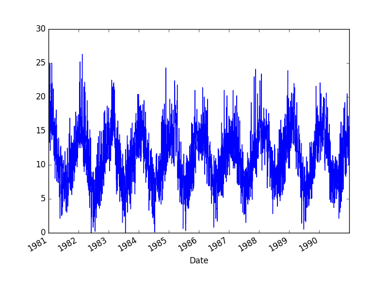
This dataset describes the minimum daily temperatures over 10 years (1981-1990) in the city Melbourne, Australia.
The units are in degrees Celsius and there are 3,650 observations. The source of the data is credited as the Australian Bureau of Meteorology.
Running the example creates a line plot of the time series.
Minimum Daily Temperatures Dataset Plot
Stop learning Time Series Forecasting the slow way!
Take my free 7-day email course and discover how to get started (with sample code).
Click to sign-up and also get a free PDF Ebook version of the course.
ARIMA Test Setup
We will use a consistent test harness to fit ARIMA models and evaluate their predictions.
First, the loaded dataset is split into a train and test dataset. The majority of the dataset is used to fit the model and the last 7 observations (one week) are held back as the test dataset to evaluate the fit model.
A walk-forward validation, or rolling forecast, method is used as follows:
Each time step in the test dataset is iterated.
Within each iteration, a new ARIMA model is trained on all available historical data.
The model is used to make a prediction for the next day.
The prediction is stored and the “real” observation is retrieved from the test set and added to the history for use in the next iteration.
The performance of the model is summarized at the end by calculating the root mean squared error (RMSE) of all predictions made compared to expected values in the test dataset.
Simple AR, MA, ARMA and ARMA models are developed. They are unoptimized and are used for demonstration purposes. You will surely be able to achieve better performance with a little tuning.
The ARIMA implementation from the statsmodels Python library is used and AR and MA coefficients are extracted from the ARIMAResults object returned from fitting the model.
The ARIMA model supports forecasts via the predict() and the forecast() functions.
Nevertheless, we will make manual predictions in this tutorial using the learned coefficients.
This is useful as it demonstrates that all that is required from a trained ARIMA model is the coefficients.
The coefficients in the statsmodels implementation of the ARIMA model do not use intercept terms. This means we can calculate the output values by taking the dot product of the learned coefficients and lag values (in the case of an AR model) and lag residuals (in the case of an MA model). For example:
1
y = dot_product(ar_coefficients, lags) + dot_product(ma_coefficients, residuals)
The coefficients of a learned ARIMA model can be accessed from aARIMAResults object as follows:
AR Coefficients: model_fit.arparams
MA Coefficients: model_fit.maparams
We can use these retrieved coefficients to make predictions using the following manual predict() function.
1
2
3
4
5
def predict(coef,history):
yhat=0.0
foriinrange(1,len(coef)+1):
yhat+=coef[i-1]*history[-i]
returnyhat
For reference, you may find the following resources useful:
In this example, we will use a simple AR(1) for demonstration purposes.
Making a prediction requires that we retrieve the AR coefficients from the fit model and use them with the lag of observed values and call the custom predict() function defined above.
Note that the ARIMA implementation will automatically model a trend in the time series. This adds a constant to the regression equation that we do not need for demonstration purposes. We turn this convenience off by setting the ‘trend’ argument in the fit() function to the value ‘nc‘ for ‘no constant‘.
The fit() function also outputs a lot of verbose messages that we can turn off by setting the ‘disp‘ argument to ‘False‘.
Running the example prints the prediction and expected value each iteration for 7 days. The final RMSE is printed showing an average error of about 1.9 degrees Celsius for this simple model.
1
2
3
4
5
6
7
8
>predicted=9.738, expected=12.900
>predicted=12.563, expected=14.600
>predicted=14.219, expected=14.000
>predicted=13.635, expected=13.600
>predicted=13.245, expected=13.500
>predicted=13.148, expected=15.700
>predicted=15.292, expected=13.000
Test RMSE: 1.928
Experiment with AR models with different orders, such as 2 or more.
Moving Average Model
The moving average model, or MA, is a linear regression model of the lag residual errors.
An MA model with a lag of k can be specified in the ARIMA model as follows:
1
model=ARIMA(history,order=(0,0,k))
In this example, we will use a simple MA(1) for demonstration purposes.
Much like above, making a prediction requires that we retrieve the MA coefficients from the fit model and use them with the lag of residual error values and call the custom predict() function defined above.
The residual errors during training are stored in the ARIMA model under the ‘resid‘ parameter of the ARIMAResults object.
Running the example prints the predictions and expected values each iteration for 7 days and ends by summarizing the RMSE of all predictions.
The skill of the model is not great and you can use this as an opportunity to explore MA models with other orders and use them to make manual predictions.
1
2
3
4
5
6
7
8
>predicted=4.610, expected=12.900
>predicted=7.085, expected=14.600
>predicted=6.423, expected=14.000
>predicted=6.476, expected=13.600
>predicted=6.089, expected=13.500
>predicted=6.335, expected=15.700
>predicted=8.006, expected=13.000
Test RMSE: 7.568
You can see how it would be straightforward to keep track of the residual errors manually outside of the ARIMAResults object as new observations are made available. For example:
1
2
3
4
residuals=list()
...
error=expected-predicted
residuals.append(error)
Next, let’s put the AR and MA models together and see how we can perform manual predictions.
Autoregression Moving Average Model
We have now seen how we can make manual predictions for a fit AR and MA model.
These approaches can be put directly together to make manual predictions for a fuller ARMA model.
In this example, we will fit an ARMA(1,1) model that can be configured in an ARIMA model as ARIMA(1,0,1) with no differencing.
You can see that the prediction (yhat) is the sum of the dot product of the AR coefficients and lag observations and the MA coefficients and lag residual errors.
Again, running the example prints the predictions and expected values each iteration and the summary RMSE for all predictions made.
1
2
3
4
5
6
7
8
>predicted=11.920, expected=12.900
>predicted=12.309, expected=14.600
>predicted=13.293, expected=14.000
>predicted=13.549, expected=13.600
>predicted=13.504, expected=13.500
>predicted=13.434, expected=15.700
>predicted=14.401, expected=13.000
Test RMSE: 1.405
We can now add differencing and show how to make predictions for a complete ARIMA model.
Autoregression Integrated Moving Average Model
The I in ARIMA stands for integrated and refers to the differencing performed on the time series observations before predictions are made in the linear regression model.
When making manual predictions, we must perform this differencing of the dataset prior to calling the predict() function. Below is a function that implements differencing of the entire dataset.
1
2
3
4
5
6
def difference(dataset):
diff=list()
foriinrange(1,len(dataset)):
value=dataset[i]-dataset[i-1]
diff.append(value)
returnnumpy.array(diff)
A simplification would be to keep track of the observation at the oldest required lag value and use that to calculate the differenced series prior to prediction as needed.
This difference function can be called once for each difference required of the ARIMA model.
In this example, we will use a difference level of 1, and combine it with the ARMA example in the previous section to give us an ARIMA(1,1,1) model.
You can see that the lag observations are differenced prior to their use in the call to the predict() function with the AR coefficients. The residual errors will also be calculated with regard to these differenced input values.
Running the example prints the prediction and expected value each iteration and summarizes the performance of all predictions made.
1
2
3
4
5
6
7
8
>predicted=11.837, expected=12.900
>predicted=13.265, expected=14.600
>predicted=14.159, expected=14.000
>predicted=13.868, expected=13.600
>predicted=13.662, expected=13.500
>predicted=13.603, expected=15.700
>predicted=14.788, expected=13.000
Test RMSE: 1.232
Summary
In this tutorial, you discovered how to make manual predictions for an ARIMA model with Python.
Specifically, you learned:
How to make manual predictions for an AR model.
How to make manual predictions for an MA model.
How to make manual predictions for an ARMA and ARIMA model.
Do you have any questions about making manual predictions?
Ask your questions in the comments below and I will do my best to answer.
Want to Develop Time Series Forecasts with Python?
Really appreciate for this article, I’ve got one question: in this example, why do we use an iterative way to determine the ARIMA parameters, can we fix the model parameters before the loop in test dataset and then doing the validation process?
Thanks for the feedback, Jason, what I meant before is:
…
for t in range(len(test)):
model = ARIMA(history, order=(1,1,1))
…
we see that in each loop, we train the model again and get a new set of parameters. Why not train the model just based on the training set and all parameters in the model is fixed, then loop for all test set and validate the error for each of them.
Thanks a lot Jason.
Nice example from that link. I find that there’re plenty of quite useful and interesting information from your posts, I will go through others and post questions (if I have).
Again, thanks for the work, great job. 🙂
Let’s say I have two data points in a week recorded over several years, for example data from Monday and Friday. Would this affect the model? Would this be relevant for the difference function?
I have several ARIMA tutorials read on this site. Some use the difference function some not- like the parameter tunings. When do I need the difference function.
Since the dataset seems to have strong seasonality, in this case, do we need to first decompose the data by removing the seasonality factor, and then, applying models such as ARIMA?
Thanks for all the ARIMA tutorials! I’m preparing to analyze some gait data from a biomechanics lab I worked in last summer and they’re helping me to get to hang of the model.
Imagine a scenario where we are using the fitted ARIMA model i.e. the coefficients on a new dataset (out of sample). Calculating the AR part is easy. Use the previous data of length ‘p’ (history). Whereas for the MA part, one needs the residuals for past ‘q’ values. Without fitting for the new data seen, how are the the residuals calculated for the new data. Do we use the residuals found in the training data? This is useful for for ARIMA models with q>0 (i.e. having MA coefficients).
thanks for post, it is helpful.
But I have question, why the history data need to append test data for each loop:
model = ARIMA(history, order=(1,0,0))
obs = test[t]
history.append(obs)
If I do’t know the test data value, for example just predict 6 month or 1 years days(365 days range) value, how to use the model to predict. Just like machine learning, used the train set to train model, and predict new data.
Thanks a lot for these ARIMA posts, I know close to nothing about time series and I’m learning this stuff to work on a project to find a cross-correlation matrix. I need to pre-whiten the data and I used your tutorial to fit a model to one of my series. Next I have to apply this model (filter) to another series and I was wondering if you could elaborate on how to do that using predict. I’ve been scouring the internet for some material, and I don’t know what exactly the contents and format of the ‘params’ field is supposed to be.
Bonjour, est-il possible d’intégrer d’autres variables dans le modèle ARIMA pour faire de la prédiction ?
Je n etrouve pas de réponses concernant cette question.
Here in example you said 3650 observations and have taken last 7 days for test set.. I am lil confused about my data set. I have weekly data of 7 weather parameters for 30 years. How can I select the training and test set?
I tried both your method to manually predict the series (which I think correct) and statsmodels’ .predict(). Do you have an explanation on why there are not exactly same? statsmodels is not that clear about how they perform predictions. Thanks!
I have a question, how do they acf and pacf were obtained here? I have a similar dataset with almost 1100 observations, and based on my acf and pacf, I have a significant lag from 1 to 27 for the acf. I want to know also if there is a limitation for the ARIMA model when we have those high values. Thanks
hi,I think there is a big error in the ARIMA model about the difference.
When we use AIRMA(p,d,q), if d not equal to 0, the model has done the difference step.
So the predict result data also has been diffenenced, so we need to restore the data.
But the restored result (no difference) is wrong. The predict error is very big.
In your many ARIMA examples, such as ARIMA(5,1,0), the d = 1, but I didn’t find the restored difference.
If the ARIMA(5,0,0), it doesn’t need to restore the difference.
The difference I mean the parameter d in the ARIMA(p,d,q).
I think maybe the python model ARIMA has little error.
Hi, Jason, I have a question about the train and validation.
In the four examples, you split the data into train and test part. But in your prediction, you also add the data in test to the history. Is it OK to do in this way? According to my understanding, it is not right to use the data in test set.
I saw the link. It is detailed. I also checked other web pages. It seems that “walk forward validation ” is uncommon in machine learning. If we want to compare the result with other methods. What we should do?
If we use other complex methods and use “walk forward validation”, it will wast a lot of time to train the model.
This is great, thank you! I’ve been looking for a way to manually calculate prediction from parameters because I need to save parameters for forecasting in another context. And I just couldn’t find any documentation that convinced me how to do it… so thanks for this!
Firstly, thanks for the tutorial. I have a couple of questions in my mind. Firstly, if I do multi-step ahead forecasting and defining AR and MA terms with some number means that the model looks back that amount out of back steps and do the forecast for the future? If I introduce the whole historical time series to the model, how the model uses that whole historical data to do multi-step ahead forecasting? how the coefficients in the AR and MA terms are updated? I would very thankful If I understand them.
Thank you for the tutorial! I have a question about settting yhat. What would yhat equal in the (0,0,0), (0, 1, 1), (1,1,0), and (0,1,0) cases and, for those cases, what parameters should we use for the predict function?
So say I have a 0,1,0 Arima model. I need to have a constant term to be able to run it. How should I incorporate the constant term into the predict function? For the 0,1,0 case and other cases as well?
from statsmodels.tsa.arima_model import ARIMA
from sklearn.metrics import mean_squared_error
train= training_set[‘Close’].values.reshape(-1, 1) #reshaping training values
test = test_set.values.reshape(-1, 1)
history = [x for x in train]
predictions = list()
for t in range(len(test)):
model = ARIMA(history, order=(1,2,1))
model_fit = model.fit(trend=’nc’, disp=False)
ar_coef, ma_coef = model_fit.arparams, model_fit.maparams
resid = model_fit.resid
diff = difference(history)
yhat = history[-1] + predict(ar_coef, diff) + predict(ma_coef, resid)
predictions.append(yhat)
obs = test[t]
history.append(obs)
print(‘>predicted=%.3f, expected=%.3f’ % (yhat, obs))
rmse = sqrt(mean_squared_error(test, predictions))
print(‘Test RMSE: %.3f’ % rmse)
~/anaconda3/lib/python3.7/site-packages/statsmodels/tsa/arima_model.py in _fit_start_params_hr(self, order, start_ar_lags)
546 return start_params
547
–> 548 def _fit_start_params(self, order, method, start_ar_lags=None):
549 if method != ‘css-mle’: # use Hannan-Rissanen to get start params
550 start_params = self._fit_start_params_hr(order, start_ar_lags)
ValueError: The computed initial MA coefficients are not invertible
You should induce invertibility, choose a different model order, or you can
pass your own start_params.
Hi sir, i have problem with forecasting between using this manual predicting and using the library..
I compared the 2 result but it showed different result.
I use this model fitting :
model_fit = model.fit(trend=’nc’, disp=False). the library model i used show constant result . For example [10.234,10.235,10.235,….10.235,] . Can you help me please 🙂
I wonder that why we don’t use constanta in this tutorial and why disp= False?. I tried to make the parameter same but the result show different to the forecast.
My data has been preprocessed to a range of -1 and 1. I’m doing a walk-forward validation
for ARIMA and the model would predict extremely high values outside this range for some observations.


Hi Jason,
Thanks for this tutorial.
Now the error occure as follow, Please advise me about it.
I think also that the code do not have an error.
—> 23 model_fit = model.fit(trend=’nc’, disp=False)
ValueError: could not convert string to float: ?0.2
thanks
Open the downloaded data file and delete all instances of the “?” character.
It worked fine.
I did not think that it was caused by converting the file to CSV.
Thank you, Jason.
Glad to hear it!
Hi Jason
Really appreciate for this article, I’ve got one question: in this example, why do we use an iterative way to determine the ARIMA parameters, can we fix the model parameters before the loop in test dataset and then doing the validation process?
Thanks a lot for some more insights on it.
I’m not sure what you mean by iterative? Can you please elaborate?
Thanks for the feedback, Jason, what I meant before is:
…
for t in range(len(test)):
model = ARIMA(history, order=(1,1,1))
…
we see that in each loop, we train the model again and get a new set of parameters. Why not train the model just based on the training set and all parameters in the model is fixed, then loop for all test set and validate the error for each of them.
Thanks again for your reply.
You can, but if we have new data (e.g. it is the next month and a new observation is available) then we should use it.
That is what we are simulating here. It is called walk forward validation:
https://machinelearningmastery.com/backtest-machine-learning-models-time-series-forecasting/
Thanks a lot Jason.
Nice example from that link. I find that there’re plenty of quite useful and interesting information from your posts, I will go through others and post questions (if I have).
Again, thanks for the work, great job. 🙂
Thanks Luca!
Let’s say I have two data points in a week recorded over several years, for example data from Monday and Friday. Would this affect the model? Would this be relevant for the difference function?
It may, it depends on the problem.
I have several ARIMA tutorials read on this site. Some use the difference function some not- like the parameter tunings. When do I need the difference function.
When you have a trend, please read this:
https://machinelearningmastery.com/difference-time-series-dataset-python/
Hi Jason
Since the dataset seems to have strong seasonality, in this case, do we need to first decompose the data by removing the seasonality factor, and then, applying models such as ARIMA?
Thanks
It would be a good idea to seasonally adjust the dataset first:
https://machinelearningmastery.com/time-series-seasonality-with-python/
Hi Jason,
Thanks for all the ARIMA tutorials! I’m preparing to analyze some gait data from a biomechanics lab I worked in last summer and they’re helping me to get to hang of the model.
Consider a neural net model?
Hi Jason,
Imagine a scenario where we are using the fitted ARIMA model i.e. the coefficients on a new dataset (out of sample). Calculating the AR part is easy. Use the previous data of length ‘p’ (history). Whereas for the MA part, one needs the residuals for past ‘q’ values. Without fitting for the new data seen, how are the the residuals calculated for the new data. Do we use the residuals found in the training data? This is useful for for ARIMA models with q>0 (i.e. having MA coefficients).
Good question. The ARIMA model will make these available in “model_fit.resid” I believe.
thanks for post, it is helpful.
But I have question, why the history data need to append test data for each loop:
model = ARIMA(history, order=(1,0,0))
obs = test[t]
history.append(obs)
If I do’t know the test data value, for example just predict 6 month or 1 years days(365 days range) value, how to use the model to predict. Just like machine learning, used the train set to train model, and predict new data.
Because we are evaluating the model using walk-forward validation:
https://machinelearningmastery.com/backtest-machine-learning-models-time-series-forecasting/
Hey Jason,
Thanks a lot for these ARIMA posts, I know close to nothing about time series and I’m learning this stuff to work on a project to find a cross-correlation matrix. I need to pre-whiten the data and I used your tutorial to fit a model to one of my series. Next I have to apply this model (filter) to another series and I was wondering if you could elaborate on how to do that using predict. I’ve been scouring the internet for some material, and I don’t know what exactly the contents and format of the ‘params’ field is supposed to be.
Thanks a lot!
This might be a good place to start with time series:
https://machinelearningmastery.com/start-here/#timeseries
I don’t have material on how to whiten a time series, sorry.
Bonjour, est-il possible d’intégrer d’autres variables dans le modèle ARIMA pour faire de la prédiction ?
Je n etrouve pas de réponses concernant cette question.
Yes, it is called exogenous variables.
Sorry, I don’t have an example.
Hi! How can I predct for example 20 reading forward?
mod =ARIMA(X, order=(self.p, self.d, self.q)
res = mod.fit()
res.forecast(20)
Perhaps this post will help:
https://machinelearningmastery.com/make-sample-forecasts-arima-python/
Hello Jason,
Here in example you said 3650 observations and have taken last 7 days for test set.. I am lil confused about my data set. I have weekly data of 7 weather parameters for 30 years. How can I select the training and test set?
Perhaps use a little trial and error and see how much history is required to fit a skilful model with your specific data.
This post might give you ideas:
https://machinelearningmastery.com/sensitivity-analysis-history-size-forecast-skill-arima-python/
I tried both your method to manually predict the series (which I think correct) and statsmodels’ .predict(). Do you have an explanation on why there are not exactly same? statsmodels is not that clear about how they perform predictions. Thanks!
The predict() and the forecast() functions should return the same results.
Learn how to use them here:
https://machinelearningmastery.com/make-sample-forecasts-arima-python/
I have a question, how do they acf and pacf were obtained here? I have a similar dataset with almost 1100 observations, and based on my acf and pacf, I have a significant lag from 1 to 27 for the acf. I want to know also if there is a limitation for the ARIMA model when we have those high values. Thanks
I used the statsmodels plot functions.
hi,I think there is a big error in the ARIMA model about the difference.
When we use AIRMA(p,d,q), if d not equal to 0, the model has done the difference step.
So the predict result data also has been diffenenced, so we need to restore the data.
But the restored result (no difference) is wrong. The predict error is very big.
In your many ARIMA examples, such as ARIMA(5,1,0), the d = 1, but I didn’t find the restored difference.
If the ARIMA(5,0,0), it doesn’t need to restore the difference.
The difference I mean the parameter d in the ARIMA(p,d,q).
I think maybe the python model ARIMA has little error.
The model will invert the difference (if needed) when a prediction is made.
Hi, Jason, I have a question about the train and validation.
In the four examples, you split the data into train and test part. But in your prediction, you also add the data in test to the history. Is it OK to do in this way? According to my understanding, it is not right to use the data in test set.
Another question is about the prediction. According to the document (https://www.statsmodels.org/dev/generated/statsmodels.tsa.arima_model.ARMAResults.forecast.html#statsmodels.tsa.arima_model.ARMAResults.forecast), we can predict the future in many steps (not only 1). Why you do not use the steps directly?
Yes, this is called walk forward validation, more here:
https://machinelearningmastery.com/backtest-machine-learning-models-time-series-forecasting/
I saw the link. It is detailed. I also checked other web pages. It seems that “walk forward validation ” is uncommon in machine learning. If we want to compare the result with other methods. What we should do?
If we use other complex methods and use “walk forward validation”, it will wast a lot of time to train the model.
Thanks.
It is common in time series forecasting problems.
Other methods should use the approach, and if they do not, such as using cross validation, their results are almost certainly invalid.
How can I calculate training error for time series?
Typically we use mean squared error (MSE) or root mean squared error (RMSE).
This is great, thank you! I’ve been looking for a way to manually calculate prediction from parameters because I need to save parameters for forecasting in another context. And I just couldn’t find any documentation that convinced me how to do it… so thanks for this!
I’m happy it helped!
Yes we calculate RMSE but how? What will be the actual and predicted values?
You can use sklearn to calculate RMSE.
Calculate MSE, then take the square root:
https://scikit-learn.org/stable/modules/generated/sklearn.metrics.mean_squared_error.html
Hi Jason,
Firstly, thanks for the tutorial. I have a couple of questions in my mind. Firstly, if I do multi-step ahead forecasting and defining AR and MA terms with some number means that the model looks back that amount out of back steps and do the forecast for the future? If I introduce the whole historical time series to the model, how the model uses that whole historical data to do multi-step ahead forecasting? how the coefficients in the AR and MA terms are updated? I would very thankful If I understand them.
Kind Regards,
Gunay
Perhaps this will help:
https://machinelearningmastery.com/make-sample-forecasts-arima-python/
Hi Jason,
Thank you for the tutorial! I have a question about settting yhat. What would yhat equal in the (0,0,0), (0, 1, 1), (1,1,0), and (0,1,0) cases and, for those cases, what parameters should we use for the predict function?
Thank you,
Emilio
I’m not sure I follow.
yhat is the prediction from the model.
The order (e.g. (0,1,0)) is the configuration of the model.
Does that help?
So say I have a 0,1,0 Arima model. I need to have a constant term to be able to run it. How should I incorporate the constant term into the predict function? For the 0,1,0 case and other cases as well?
Good question, perhaps check the source code for exactly how the statsmodels implementation incorporates the constant.
Or just use the statsmodels model directly:
https://machinelearningmastery.com/make-sample-forecasts-arima-python/
Thanks for the article. Can I ask then how to use this model to predict future days? This practice shows prediction for current data.
TQ
Yes, I show how here:
https://machinelearningmastery.com/make-sample-forecasts-arima-python/
Thanks for writing this. I always enjoy your articles.
How would this work for higher order models like ARIMA(4,1,1)?
Same general idea, although it might be easier to resort to the forecast() or predict() functions:
https://machinelearningmastery.com/make-sample-forecasts-arima-python/
This is my code:
from statsmodels.tsa.arima_model import ARIMA
from sklearn.metrics import mean_squared_error
train= training_set[‘Close’].values.reshape(-1, 1) #reshaping training values
test = test_set.values.reshape(-1, 1)
history = [x for x in train]
predictions = list()
for t in range(len(test)):
model = ARIMA(history, order=(1,2,1))
model_fit = model.fit(trend=’nc’, disp=False)
ar_coef, ma_coef = model_fit.arparams, model_fit.maparams
resid = model_fit.resid
diff = difference(history)
yhat = history[-1] + predict(ar_coef, diff) + predict(ma_coef, resid)
predictions.append(yhat)
obs = test[t]
history.append(obs)
print(‘>predicted=%.3f, expected=%.3f’ % (yhat, obs))
rmse = sqrt(mean_squared_error(test, predictions))
print(‘Test RMSE: %.3f’ % rmse)
Output:
>predicted=3366.015, expected=3370.000
>predicted=3371.046, expected=3390.000
>predicted=3369.670, expected=3370.000
>predicted=3392.017, expected=3377.800
>predicted=3373.568, expected=3460.000
>predicted=3369.171, expected=3460.000
>predicted=3452.457, expected=3400.000
>predicted=3469.630, expected=3458.100
>predicted=3402.823, expected=3490.000
>predicted=3449.645, expected=3490.000
>predicted=3488.853, expected=3442.200
>predicted=3498.426, expected=3468.300
>predicted=3447.526, expected=3489.000
>predicted=3465.161, expected=3510.000
>predicted=3486.675, expected=3485.000
>predicted=3513.211, expected=3498.900
>predicted=3489.170, expected=3500.000
>predicted=3499.777, expected=3580.000
>predicted=3493.101, expected=3495.200
>predicted=3583.419, expected=3545.500
>predicted=3503.000, expected=3720.000
—————————————————————————
ValueError Traceback (most recent call last)
in
8 for t in range(len(test)):
9 model = ARIMA(history, order=(1,2,1))
—> 10 model_fit = model.fit(trend=’nc’, disp=False)
11 ar_coef, ma_coef = model_fit.arparams, model_fit.maparams
12 resid = model_fit.resid
~/anaconda3/lib/python3.7/site-packages/statsmodels/tsa/arima_model.py in fit(self, start_params, trend, method, transparams, solver, maxiter, full_output, disp, callback, start_ar_lags, **kwargs)
1155 arima_fit.mle_retvals = mlefit.mle_retvals
1156 arima_fit.mle_settings = mlefit.mle_settings
-> 1157
1158 return ARIMAResultsWrapper(arima_fit)
1159
~/anaconda3/lib/python3.7/site-packages/statsmodels/tsa/arima_model.py in fit(self, start_params, trend, method, transparams, solver, maxiter, full_output, disp, callback, start_ar_lags, **kwargs)
944 kwargs.setdefault(‘pgtol’, 1e-8)
945 kwargs.setdefault(‘factr’, 1e2)
–> 946 kwargs.setdefault(‘m’, 12)
947 kwargs.setdefault(‘approx_grad’, True)
948 mlefit = super(ARMA, self).fit(start_params, method=solver,
~/anaconda3/lib/python3.7/site-packages/statsmodels/tsa/arima_model.py in _fit_start_params(self, order, method, start_ar_lags)
560 pgtol=1e-7, factr=1e3,
561 bounds=bounds, iprint=-1)
–> 562 start_params = mlefit[0]
563 if self.transparams:
564 start_params = self._transparams(start_params)
~/anaconda3/lib/python3.7/site-packages/statsmodels/tsa/arima_model.py in _fit_start_params_hr(self, order, start_ar_lags)
546 return start_params
547
–> 548 def _fit_start_params(self, order, method, start_ar_lags=None):
549 if method != ‘css-mle’: # use Hannan-Rissanen to get start params
550 start_params = self._fit_start_params_hr(order, start_ar_lags)
ValueError: The computed initial MA coefficients are not invertible
You should induce invertibility, choose a different model order, or you can
pass your own start_params.
Yes, some configurations will result in an unstable model.
Hi sir, i have problem with forecasting between using this manual predicting and using the library..
I compared the 2 result but it showed different result.
I use this model fitting :
model_fit = model.fit(trend=’nc’, disp=False). the library model i used show constant result . For example [10.234,10.235,10.235,….10.235,] . Can you help me please 🙂
You might need to dig into the statsmodels source code to see what additional steps are being used.
I wonder that why we don’t use constanta in this tutorial and why disp= False?. I tried to make the parameter same but the result show different to the forecast.
We set display to False to remove the verbose output.
Hi Sir, thank you for the impact.
My data has been preprocessed to a range of -1 and 1. I’m doing a walk-forward validation
for ARIMA and the model would predict extremely high values outside this range for some observations.
Is there any reason for that?
Thank you.
Perhaps the model needs to be further tuned for your dataset?
Perhaps you need to scale data to a different range?
Perhaps try an alternate model?