
Logistic regression is one of the most popular machine learning algorithms for binary classification. This is because it is a simple algorithm that performs very well on a wide range of problems.
In this post you are going to discover the logistic regression algorithm for binary classification, step-by-step. After reading this post you will know:
- How to calculate the logistic function.
- How to learn the coefficients for a logistic regression model using stochastic gradient descent.
- How to make predictions using a logistic regression model.
This post was written for developers and does not assume a background in statistics or probability. Open a spreadsheet and follow along. If you have any questions about Logistic Regression ask in the comments and I will do my best to answer.
Kick-start your project with my new book Master Machine Learning Algorithms, including step-by-step tutorials and the Excel Spreadsheet files for all examples.
Let’s get started.
Update Nov/2016: Fixed a small typo in the update equation for b0.

Logistic Regression Tutorial for Machine Learning
Photo by Brian Gratwicke, some rights reserved.
Tutorial Dataset
In this tutorial we will use a contrived dataset.
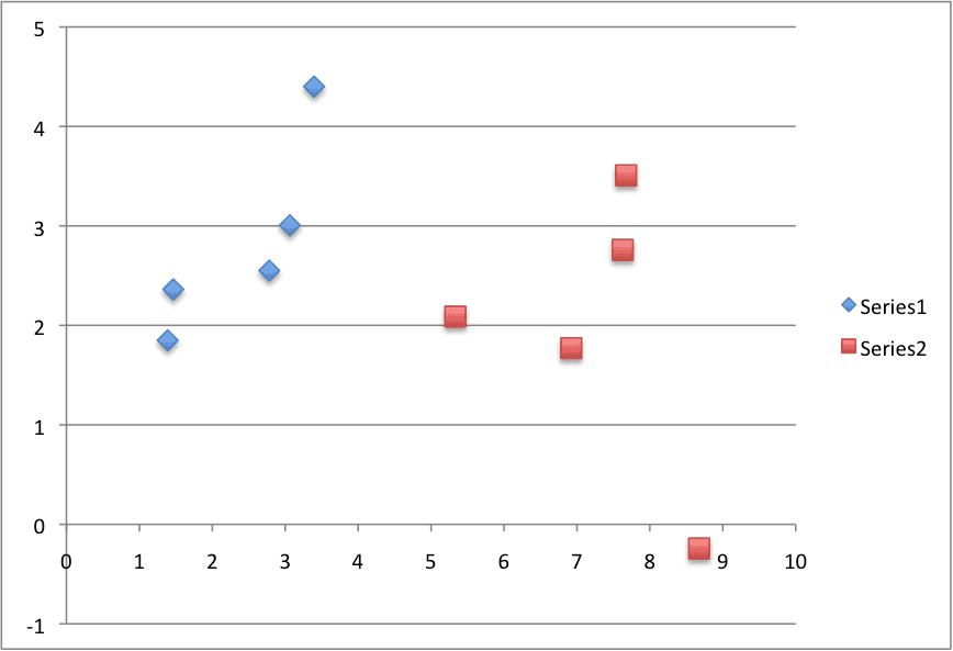
This dataset has two input variables (X1 and X2) and one output variable (Y). In input variables are real-valued random numbers drawn from a Gaussian distribution. The output variable has two values, making the problem a binary classification problem.
The raw data is listed below.
|
1 2 3 4 5 6 7 8 9 10 11 |
X1 X2 Y 2.7810836 2.550537003 0 1.465489372 2.362125076 0 3.396561688 4.400293529 0 1.38807019 1.850220317 0 3.06407232 3.005305973 0 7.627531214 2.759262235 1 5.332441248 2.088626775 1 6.922596716 1.77106367 1 8.675418651 -0.2420686549 1 7.673756466 3.508563011 1 |
Below is a plot of the dataset. You can see that it is completely contrived and that we can easily draw a line to separate the classes.
This is exactly what we are going to do with the logistic regression model.
Logistic Regression Tutorial Dataset
Logistic Function
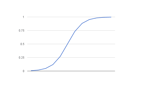
Before we dive into logistic regression, let’s take a look at the logistic function, the heart of the logistic regression technique.
The logistic function is defined as:
transformed = 1 / (1 + e^-x)
Where e is the numerical constant Euler’s number and x is a input we plug into the function.
Let’s plug in a series of numbers from -5 to +5 and see how the logistic function transforms them:
|
1 2 3 4 5 6 7 8 9 10 11 12 |
X Transformed -5 0.006692850924 -4 0.01798620996 -3 0.04742587318 -2 0.119202922 -1 0.2689414214 0 0.5 1 0.7310585786 2 0.880797078 3 0.9525741268 4 0.98201379 5 0.9933071491 |
You can see that all of the inputs have been transformed into the range [0, 1] and that the smallest negative numbers resulted in values close to zero and the larger positive numbers resulted in values close to one. You can also see that 0 transformed to 0.5 or the midpoint of the new range.
From this we can see that as long as our mean value is zero, we can plug in positive and negative values into the function and always get out a consistent transform into the new range.
Logistic Function
Get your FREE Algorithms Mind Map
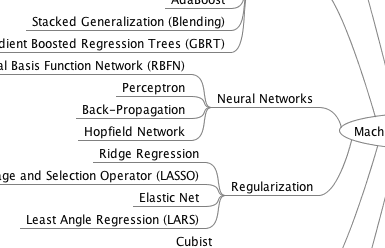
Sample of the handy machine learning algorithms mind map.
I've created a handy mind map of 60+ algorithms organized by type.
Download it, print it and use it.
Also get exclusive access to the machine learning algorithms email mini-course.
Logistic Regression Model
The logistic regression model takes real-valued inputs and makes a prediction as to the probability of the input belonging to the default class (class 0).
If the probability is > 0.5 we can take the output as a prediction for the default class (class 0), otherwise the prediction is for the other class (class 1).
For this dataset, the logistic regression has three coefficients just like linear regression, for example:
output = b0 + b1*x1 + b2*x2
The job of the learning algorithm will be to discover the best values for the coefficients (b0, b1 and b2) based on the training data.
Unlike linear regression, the output is transformed into a probability using the logistic function:
p(class=0) = 1 / (1 + e^(-output))
In your spreadsheet this would be written as:
p(class=0) = 1 / (1 + EXP(-output))
Logistic Regression by Stochastic Gradient Descent
We can estimate the values of the coefficients using stochastic gradient descent.
This is a simple procedure that can be used by many algorithms in machine learning. It works by using the model to calculate a prediction for each instance in the training set and calculating the error for each prediction.
We can apply stochastic gradient descent to the problem of finding the coefficients for the logistic regression model as follows:
Given each training instance:
- Calculate a prediction using the current values of the coefficients.
- Calculate new coefficient values based on the error in the prediction.
The process is repeated until the model is accurate enough (e.g. error drops to some desirable level) or for a fixed number iterations. You continue to update the model for training instances and correcting errors until the model is accurate enough orc cannot be made any more accurate. It is often a good idea to randomize the order of the training instances shown to the model to mix up the corrections made.
By updating the model for each training pattern we call this online learning. It is also possible to collect up all of the changes to the model over all training instances and make one large update. This variation is called batch learning and might make a nice extension to this tutorial if you’re feeling adventurous.
Calculate Prediction
Let’s start off by assigning 0.0 to each coefficient and calculating the probability of the first training instance that belongs to class 0.
B0 = 0.0
B1 = 0.0
B2 = 0.0
The first training instance is: x1=2.7810836, x2=2.550537003, Y=0
Using the above equation we can plug in all of these numbers and calculate a prediction:
prediction = 1 / (1 + e^(-(b0 + b1*x1 + b2*x2)))
prediction = 1 / (1 + e^(-(0.0 + 0.0*2.7810836 + 0.0*2.550537003)))
prediction = 0.5
Calculate New Coefficients
We can calculate the new coefficient values using a simple update equation.
b = b + alpha * (y – prediction) * prediction * (1 – prediction) * x
Where b is the coefficient we are updating and prediction is the output of making a prediction using the model.
Alpha is parameter that you must specify at the beginning of the training run. This is the learning rate and controls how much the coefficients (and therefore the model) changes or learns each time it is updated. Larger learning rates are used in online learning (when we update the model for each training instance). Good values might be in the range 0.1 to 0.3. Let’s use a value of 0.3.
You will notice that the last term in the equation is x, this is the input value for the coefficient. You will notice that the B0 does not have an input. This coefficient is often called the bias or the intercept and we can assume it always has an input value of 1.0. This assumption can help when implementing the algorithm using vectors or arrays.
Let’s update the coefficients using the prediction (0.5) and coefficient values (0.0) from the previous section.
b0 = b0 + 0.3 * (0 – 0.5) * 0.5 * (1 – 0.5) * 1.0
b1 = b1 + 0.3 * (0 – 0.5) * 0.5 * (1 – 0.5) * 2.7810836
b2 = b2 + 0.3 * (0 – 0.5) * 0.5 * (1 – 0.5) * 2.550537003
or
b0 = -0.0375
b1 = -0.104290635
b2 = -0.09564513761
Repeat the Process
We can repeat this process and update the model for each training instance in the dataset.
A single iteration through the training dataset is called an epoch. It is common to repeat the stochastic gradient descent procedure for a fixed number of epochs.
At the end of epoch you can calculate error values for the model. Because this is a classification problem, it would be nice to get an idea of how accurate the model is at each iteration.
The graph below show a plot of accuracy of the model over 10 epochs.
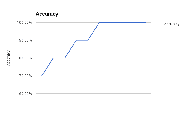
Logistic Regression with Gradient Descent Accuracy versus Iteration
You can see that the model very quickly achieves 100% accuracy on the training dataset.
The coefficients calculated after 10 epochs of stochastic gradient descent are:
b0 = -0.4066054641
b1 = 0.8525733164
b2 = -1.104746259
Make Predictions
Now that we have trained the model, we can use it to make predictions.
We can make predictions on the training dataset, but this could just as easily be new data.
Using the coefficients above learned after 10 epochs, we can calculate output values for each training instance:
|
1 2 3 4 5 6 7 8 9 10 |
0.2987569857 0.145951056 0.08533326531 0.2197373144 0.2470590002 0.9547021348 0.8620341908 0.9717729051 0.9992954521 0.905489323 |
These are the probabilities of each instance belonging to class=0. We can convert these into crisp class values using:
prediction = IF (output < 0.5) Then 0 Else 1
With this simple procedure we can convert all of the outputs to class values:
|
1 2 3 4 5 6 7 8 9 10 |
0 0 0 0 0 1 1 1 1 1 |
Finally, we can calculate the accuracy for the model on the training dataset:
accuracy = (correct predictions / num predictions made) * 100
accuracy = (10 /10) * 100
accuracy = 100%
Summary
In this post you discovered how you can implement logistic regression from scratch, step-by-step. You learned:
- How to calculate the logistic function.
- How to learn the coefficients for a logistic regression model using stochastic gradient descent.
- How to make predictions using a logistic regression model.
Do you have any questions about this post or logistic regression?
Leave a comment and ask your question, I’ll do my best to answer.
Discover How Machine Learning Algorithms Work!
See How Algorithms Work in Minutes
...with just arithmetic and simple examples
Discover how in my new Ebook:
Master Machine Learning Algorithms
It covers explanations and examples of 10 top algorithms, like:
Linear Regression, k-Nearest Neighbors, Support Vector Machines and much more...
Finally, Pull Back the Curtain on
Machine Learning Algorithms
Skip the Academics. Just Results.


Hi Jason,
Great blog! Nice job. Just wondering how to determine the form of the update equation? In this case, it’s in the form of b = b + alpha * (y – prediction) * prediction * (1 – prediction) * x. How do I know it should be like this?
Thanks.
Actually I have the same question. Plus I tried to reproduce your example but I can’t get the same (b0,b1,b2) after 10 iterations. I have instead (-0.02,0.312,-0.095)
thank you
I got the wrong value too, but i found my error.I don’t know how to descible so i leave my code, it’s coded in C++.It maybe helpful for you. Here is it:
int k = 0;
for (int j = 0; j < 100; j++) { // I forgot this loop, i added it then i got the right value.
k = 0;
while (k < 10) {
for (int i = 0; i < 3; i++){
b[i] = b[i] + alpha * (y[k] – prediction) * prediction * (1 – prediction)* x[k][i];
cout << b[i]<<"\n";
}
k++;
output = 0;
for (int i = 0; i < 3; i++)
output += b[i] * x[k][i];
prediction = 1 / (1 + exp(-output));
}
}
please send me the whole source code
Hi I managed to reproduce the same result after 10 epochs. There is a typo in the code provided here. The updating equation for:
b0 = 0.0 + 0.3 * (0 – 0.5) * 0.5 * (1 – 0.5) * 1.0
should be changed as:
b0 = b0 + 0.3 * (0 – 0.5) * 0.5 * (1 – 0.5) * 1.0
Hope this helps 🙂
Thanks Dylan, I have updated the example.
This is a great article indeed.
For the mathematical background, I referred:
“[2010] GENERATIVE AND DISCRIMINATIVE CLASSIFIERS- NAIVE BAYES AND LOGISTIC REGRESSION – Tom Mitchell”.
The weights my program finally learnt are:
[-0.48985449 0.99888324 -1.4328438 ]
My notebook can be found at:
https://j-dhall.github.io/ml/2021/02/22/logistic-regression-for-binary-classification-of-demo-data.html
Notebook: https://github.com/j-dhall/ml/blob/gh-pages/notebooks/Logistic%20Regression%20for%20Binary%20Classification%20of%20Demo%20Data.ipynb
Thanks for sharing.
I have the same question
It seems that the weight update is not right..
Old: b = b + alpha * (y – prediction) * prediction * (1 – prediction) * x
New : b = b + alpha * (y – prediction) * x
The derivative is:
http://ml-cheatsheet.readthedocs.io/en/latest/logistic_regression.html
I took the equation from AI a modern approach by norvig, not a random cheat sheet.
Thanks a lot for providing the reference. The difference comes from their different cost functions. The formula in the book –AI a modern approach– uses the quadratic cost function (y-h(x))^2. The formula in the cheat sheet uses the cross entropy as the cost function.
If a user expects the logistic regression to compute the class category value 0 and 1, the quadratic cost function makes better sense.
If a user expects the logistic regression to compute the class category probability, the cross entropy function makes better sense.
This is very interesting. Thanks.
By the way. Professor Geoffrey Hinton has the following comments when introducing the cross entropy for softmax output function in his coursera course– Neural Networks for Machine Learning — lecture 4:
• The squared error measure has some drawbacks:
– If the desired output is 1 and the actual output is 0.00000001
there is almost no gradient for a logistic unit to fix up the error.
– If we are trying to assign probabilities to mutually exclusive class
labels, we know that the outputs should sum to 1, but we are
depriving the network of this knowledge
Nicely put!
The loss function in that book seems to be at odds to other books such as “Elements of Statistical Learning”, the wikipedia, and what my common sense tells me. I find it surprising, given how popular it is. I will not say it is wrong because it works as a cost function, but it is clearly going to produce a different result than what is called “logistic regression” elsewhere, and I think there should be some mention to it in the article.
There are many ways to find coefficients for a logistic regression model.
This equation is coming from the perspective where the loss is calculated as (y – y_hat)^2 and gradient computed on the basis of this loss function.
This is explained in the book by Prof Peter Norvig, Artificial Intelligence – A modern approach, page 726(third edition)
You can also compute the gradients based on cross entropy loss. Both should converge to the same solution.
Hi,
I can’t reproduce the value of your 10th iteration of vector (b0,b1,b2)
can you explain again the iteration process.
thank you
Hi all,
In this blog it is written that the coefficients calculated after 10
epochs of stochastic gradient descent are:
b0 = -0.4066054641
b1 = 0.8525733164
b2 = -1.104746259
Through my understanding I have a matrix of inputs of size (3×10,
x1,x2,y1) and weight matrix (3×10, b0,b1,b2) after 10 epochs.
My doubts is that this learned coefficients will only be for that
particular input vector (say first input) or for all the rest of the
input?
1) If it is for single input vector then, while testing the model that were
build using above described method, how to pass any unseen input? Will every
input pass through whole neurons?
2) If not then how to compute the coefficient?
This article was very well-written and helped me immensely in understanding logistic regression. Thank you so much.
I’m glad to hear it Tom.
Jason, elucidated it very well! Clean and neat, I have come across many Blogs on ML. But yours always keep me hooked to your Knowledge Materials.
Thanks Karthik.
I strongly agree
Thanks!
Hi Jason, I have some questions for you.
[1] How can we produce the line separating these two classes? I have tried using ‘B0’ as the y-intercept, and ‘B1’ as the gradient. I am not sure if this is the case as ‘B2’ is left out of the equation.
Example:
Assuming the separator line will be from (x0,y0) to (x1,y1)
**Using the values of B0 and B1 after 10 epochs**
when x0 = minX1 = 1.38807
y0 = 1.38807(0.85257334) + (-0.40660548) = 0.77682614
when x1 = maxX1 = 8.675419
y1 = 8.675419(0.8527334) + (-0.40660548) = 6.9898252
This line (1.38807, 0.77682614) to (8.675419,6.9898252) perfectly separates the two classes, however upon increasing the number of epochs, the gradient changes and therefore produces false positives.
Any ideas please?
Thanks in advance for your help
Hi Dylan, I agree with your intuition that the regression line best separates the two classes. Drawing it should draw the class boundary for the classifier I would expect.
It is possible that additional training is overfitting or that online gradient descent is resulting in noisy changes to the line.
Really helpful, very nice explanation ,thank you so much.
what’s the main use of logistic regression Algorithm which was explained by you ….?
Great question Harish,
Logistic regression is for binary classification problems, ideally where we can separate the 2 classes by a line or hyperplane.
If logistic regression works well on your problem, use it. If not, you may need to move on to more advanced methods, even non-linear methods.
How would the approach vary if you were using poisson or log binomial regression to model binary outcomes?
1)whats the use of calculating new coefficients i am unable to understand where these coefficients used??
2)How do you draw the accurate graph and values of MAKE PREDICTION??
Hi Harish, coefficients are used to make predictions on new data.
We use the prediction equation with the coefficients and the input values in order to make predict the class of a new piece of data.
If we make predictions on test data, then calculate the error of those predictions we can make a graph of accuracy each time the coefficients are updated. That is how the graph is created.
Hi Jason – Thanks for the article. It has been helpful but can you please explain the iteration process for each Epoch?
I don’t get the same values for the 10th Epoch. It isn’t clear if you are moving to the corresponding x1, x2 and Y values for each training instance in the Prediction and the calculation of the coefficients. For example the 2nd training instance I am assuming:
prediction = 1 / (1 + e^(-(-0.0375 + -1.043*2.7810836 + -0.0956*2.550537003)))
=0.3974
b0 = b0 + 0.3 * (0 – 0.0375) * 0.0375 * (1 – 0.0375) * 1.0
b1 = b1 + 0.3 * (0 – 0.0375) * 0.0375 * (1 – 0.0375) * 1.4655
b2 = b2 + 0.3 * (0 – 0.0375) * 0.5 * (1 – 0.0375) * 2.3621
I repeat this step another 8 times updating the y,X1 and X2 values but they dont match yours. I’d be grateful if you could point out there’s something I’m missing or post your results for each training instance.
Sorry the prediction line should read:
prediction = 1 / (1 + e^(-(-0.0375 + -1.043*1.4655+ -0.0956*2.3621)))
You are right, but you missing the understanding of one epoch.
The first time, i did like you did : Updating 10 times b0, b1 and b2 and i did not have the result expected.
You have to update 10 * 10 times your b0, b1 and b2 :
One epoch is a complet turn of your data training.
Do what you did in your post, but repeat it 10 times and you’ll have the same result as the tutorial.
I did a C Program, I post the code here :
#include
#include
#include
float x1[10] = {2.7810836,
1.465489372,
3.396561688,
1.38807019,
3.06407232,
7.627531214,
5.332441248,
6.922596716,
8.675418651,
7.673756466
};
float x2[10] = {2.550537003,
2.362125076,
4.400293529,
1.850220317,
3.005305973,
2.759262235,
2.088626775,
1.77106367,
-0.2420686549,
3.508563011
};
int y_1[10] = {0,0,0,0,0,1,1,1,1,1};
float b0 = 0.00f;
float b1 = 0.00f;
float b2 = 0.00f;
float b[3];
float prediction = 0;
float output = 0;
int main()
{
int epoch = 0;
float alpha = 0.3;
while (epoch < 10)
{
int i = 0;
while (i < 10)
{
// CALCULATE PREDICTION
output = b0 + (b1 * x1[i]) + (b2 * x2[i]);
prediction = 1/(1 + exp(-output));
printf("Prediciton = %lf\n", prediction);
// AFFINEMENT DES COEFFICIENTS
b0 = b0 + alpha * (y_1[i] – prediction) * prediction * (1 – prediction) * 1.00f;
b1 = b1 + alpha * (y_1[i] – prediction) * prediction * (1 – prediction) * x1[i];
b2 = b2 + alpha * (y_1[i] – prediction) * prediction * (1 – prediction) * x2[i];
printf("New : b0 = %lf | b1 = %lf | b2 = %lf\n\n", b0, b1, b2);
i++;
}
epoch++;
}
int i = 0;
while (i < 10)
{
output = b0 + (b1 * x1[i]) + (b2 * x2[i]);
prediction = 1/(1 + exp(-output));
printf("Prediciton = %lf\n", prediction);
i++;
}
return 0;
}
Dear Jason and Alexander,
I have tried to execute the C code but in MATLAB, however, I got totally different results! Any idea why?
I posted the MATLAB code below, please note that each epoch is saved to the prediction(i,j) array column by column
clear all,
X1 = [2.7810836, 1.465489372, 3.396561688, 1.38807019, 3.06407232, 7.627531214, 5.332441248, 6.922596716, 8.675418651, 7.673756466];
X2 = [2.550537003, 2.362125076, 4.400293529, 1.850220317, 3.005305973, 2.759262235, 2.088626775, 1.77106367, -0.2420686549, 3.508563011];
y = [0,0,0,0,0,1,1,1,1,1];
%initialize the variables
b0=0;
b1=0;
b2=0;
epochs =10 ; % epochs number ,, how many times it will repeat before selecting the final values of b0…bn
alpha=0.3; % the learning rate
prediction=[]; % an array for the predictions per each iteration per each data entry
for i = 1:epochs %the outer loop where it will work per each entry in the dataset
for j = 1:length (X1)
pred =(1/(1+ exp (- (b0+ (b1* X1(i)) + (b2*X2(i))))));
b0 = b0 + alpha * (y(i) – pred) * pred* (1 – pred) * 1;
b1 = b1 + alpha * (y(i) – pred) * pred* (1 – pred) * X1(i);
b2 = b2 + alpha * (y(i) – pred) * pred* (1 – pred) * X2(i);
display (b0);
display (b1);
display (b2);
prediction(i,j)=pred;
end
end
disp (‘____The Predictions are__________’);
for i= 1:length (X1)
pred =(1/(1+ exp (- (b0+ (b1* X1(i)) + (b2*X2(i))))));
disp (pred);
end
Solved it!
I had to replace the i in the inner loops with j
Error part:
pred =(1/(1+ exp (- (b0+ (b1* X1(i)) + (b2*X2(i))))));
b0 = b0 + alpha * (y(i) – pred) * pred* (1 – pred) * 1;
b1 = b1 + alpha * (y(i) – pred) * pred* (1 – pred) * X1(i);
b2 = b2 + alpha * (y(i) – pred) * pred* (1 – pred) * X2(i);
Correct part:
pred =(1/(1+ exp (- (b0+ (b1* X1(j)) + (b2*X2(j))))));
b0 = b0 + alpha * (y(j) – pred) * pred * (1 – pred) * 1;
b1 = b1 + alpha * (y(j) – pred) * pred * (1 – pred) * X1(j);
b2 = b2 + alpha * (y(j) – pred) * pred * (1 – pred) * X2(j);
Well done, happy to hear that!
Perhaps the difference in precision across the platforms/libraries? If so, this is common.
Hi Jack,
Yes, the process is repeated, enumerating each training example. The coefficients (b0, b1, b2) output from the previous iteration are used as inputs in the subsequent iteration.
Does that help? Is there a specific aspect I can make clearer?
I provide the fully working example and spreadsheet with my book if that helps.
Hi Jason,
Thanks for this, it’s really helpful. I just have two questions.
1. About the meaning of probability,
In the beginning you said, ‘If the probability is > 0.5 we can take the output as a prediction for the default class (class 0)’; however the IF statement states that ‘prediction = IF (output 0.5 means that the instance belongs to class 0. May you please correct me :).
2. ‘At the end of epoch you can calculate error values for the model’
Do we do this by testing each instance in the training set using coefficients obtained from the last instance during training, and check how many are correctly classified vs those incorrectly classified to get the error error of the model ?.
Thanks for your help.
Hi Ntate,
Yes, here the default class is class 1. If P > 0.5, then predict class 1.
Models are generally trained on a training dataset and evaluated on a test or validation dataset.
Does that help?
Hi Jason
Thank you for the feedback. Yes it helps. I love you articles.
Regards,
Ntate
Glad to hear it.
Hi Jason,
I noticed you assigned alpha as 0.3 and stated that a “good” value is between 0.1 – 0.3.
b = b + alpha * (y – prediction) * prediction * (1 – prediction) * x
Can you define why the range between 0.1 – 0.3 are good values? also, is there another way to determine alpha?
regards,
Trial and error is the best away to configure alpha.
My suggestion is based on observations.
Thank you.Helepd me in understanding it easily
Thanks, I’m glad to hear that.
I’ve some categorical and ordinal variables as independent variables. Do I need to normalise them for logistic regression? If yes, which normalisation?
I would recommend converting the categorical variables to integer encoded or one hot encoded first. Then consider standardizing or normalizing the real-valued variables.
Hey Jason,
I hope that you can help me out. I just loaded the dataset into a pandas dataframe and run over the values with the given functions in this article. But somehow I do not get the same results. Can you tell me why?
b0 = 0.0
b1 = 0.0
b2 = 0.0
alpha = 0.3
for i in range(10):
print(‘epoche ‘+str(i))
for j in range(10):
prediction = 1/(1+math.exp(-(b0+b1*df.X1[j]+0*df.X2[j])))
b0 = b0 + alpha*(df.Y[j]-prediction)*prediction*(1-prediction)*1
b1 = b1 + alpha*(df.Y[j]-prediction)*prediction*(1-prediction)*df.X1[j]
b2 = b2 + alpha*(df.Y[j]-prediction)*prediction*(1-prediction)*df.X2[j]
print(j,’b0:’+str(b0),’b1:’+str(b1),’b2:’+str(b2),’prediction:’,str(prediction))
epoche 0
0 b0:-0.0375 b1:-0.104290635 b2:-0.0956451376125 prediction: 0.5
1 b0:-0.0711363539015 b1:-0.153584354155 b2:-0.175098412628 prediction: 0.4525589342855867
2 b0:-0.0956211308566 b1:-0.2367484095 b2:-0.282838618223 prediction: 0.3559937888383731
3 b0:-0.12398808955 b1:-0.276123739244 b2:-0.335323741529 prediction: 0.3955015163005356
4 b0:-0.140423954937 b1:-0.326484419432 b2:-0.384718545948 prediction: 0.27487029790669615
5 b0:-0.122884891209 b1:-0.192704663377 b2:-0.336323669765 prediction: 0.06718893790753155
6 b0:-0.0812720241683 b1:0.0291935052754 b2:-0.24940992148 prediction: 0.24040302936619257
7 b0:-0.0461629882724 b1:0.27223920187 b2:-0.187229583516 prediction: 0.5301690178124752
8 b0:-0.0439592934139 b1:0.291357177347 b2:-0.187763028966 prediction: 0.9101629406368437
9 b0:-0.041234497312 b1:0.312266599052 b2:-0.178202910151 prediction: 0.8995147707414556
epoche 1
0 b0:-0.0854175615843 b1:0.189389803607 b2:-0.290893450483 prediction: 0.6957636219000934
1 b0:-0.126132084903 b1:0.129723102398 b2:-0.387066246971 prediction: 0.5478855806515489
2 b0:-0.168426127803 b1:-0.013931223349 b2:-0.573172450262 prediction: 0.5779785060018552
3 b0:-0.202118039235 b1:-0.0606979612511 b2:-0.635509909311 prediction: 0.4531965138273989
4 b0:-0.231317727075 b1:-0.150167916514 b2:-0.723263905585 prediction: 0.40417453404597653
5 b0:-0.192771357535 b1:0.143845720337 b2:-0.616904363818 prediction: 0.20153497961346012
6 b0:-0.16786327908 b1:0.2766665853 b2:-0.564880684243 prediction: 0.6397495977782179
7 b0:-0.162238550103 b1:0.315604315639 b2:-0.554918931099 prediction: 0.8516230388309892
8 b0:-0.160844460322 b1:0.327698628134 b2:-0.555256396538 prediction: 0.9292852140544192
9 b0:-0.158782126878 b1:0.34352447273 b2:-0.548020569702 prediction: 0.913238571936509
epoche 2
0 b0:-0.203070195453 b1:0.220355651541 b2:-0.660978927394 prediction: 0.6892441807751586
1 b0:-0.242672456027 b1:0.162318959562 b2:-0.754524420162 prediction: 0.5299288459930025
2 b0:-0.284900459421 b1:0.0188889410738 b2:-0.940340030239 prediction: 0.5765566602275273
3 b0:-0.317036444837 b1:-0.0257180623077 b2:-0.999798683361 prediction: 0.43568790553413944
4 b0:-0.346058130501 b1:-0.114642606031 b2:-1.08701772863 prediction: 0.4023126069119149
5 b0:-0.305303900258 b1:0.196211557251 b2:-0.974566120208 prediction: 0.22784879089424026
6 b0:-0.284135730542 b1:0.309089578586 b2:-0.930353714163 prediction: 0.6772107084944106
7 b0:-0.279392082974 b1:0.341927937662 b2:-0.921952412292 prediction: 0.8647793818147672
8 b0:-0.278250718608 b1:0.351829751376 b2:-0.922228700829 prediction: 0.9362537346812636
9 b0:-0.276418730838 b1:0.365887979368 b2:-0.915801056304 prediction: 0.9184600339928451
epoche 3
0 b0:-0.320829240308 b1:0.242378639814 b2:-1.02907170403 prediction: 0.6772464757372858
1 b0:-0.358962425423 b1:0.186494862307 b2:-1.11914705682 prediction: 0.5085926740259167
2 b0:-0.400784178807 b1:0.0444446970373 b2:-1.30317504761 prediction: 0.5681921310493052
3 b0:-0.431106414978 b1:0.00235530491457 b2:-1.35927786503 prediction: 0.4160301017601509
4 b0:-0.459481564543 b1:-0.0845882054421 b2:-1.4445538715 prediction: 0.39558638097213306
5 b0:-0.417358455079 b1:0.236707126821 b2:-1.32832516633 prediction: 0.24886389211209164
6 b0:-0.398407914119 b1:0.337759773107 b2:-1.28874455908 prediction: 0.6994895638042464
7 b0:-0.394265226466 b1:0.36643792905 b2:-1.28140759549 prediction: 0.8743265198068555
8 b0:-0.393309643975 b1:0.374728007212 b2:-1.28163891205 prediction: 0.9418454578963239
9 b0:-0.391663361645 b1:0.387361176894 b2:-1.27586282676 prediction: 0.9228889145563345
epoche 4
0 b0:-0.436106966113 b1:0.26375979738 b2:-1.38921788451 prediction: 0.6649919679911412
1 b0:-0.472655267001 b1:0.210198650866 b2:-1.47554954252 prediction: 0.4876100903262518
2 b0:-0.514052259808 b1:0.0695912110969 b2:-1.65770846209 prediction: 0.5600333525763922
3 b0:-0.542575863527 b1:0.029998447064 b2:-1.7104834132 prediction: 0.39712596044478815
4 b0:-0.570332853627 b1:-0.0550509779888 b2:-1.79390166134 prediction: 0.38920422454205744
5 b0:-0.52713220805 b1:0.274463294611 b2:-1.67469975148 prediction: 0.2708654841988902
6 b0:-0.510039576896 b1:0.365608746016 b2:-1.63899962439 prediction: 0.7183774008591356
7 b0:-0.506411991601 b1:0.390721056064 b2:-1.63257493987 prediction: 0.8829763460926162
8 b0:-0.505614321279 b1:0.397641180051 b2:-1.63276803085 prediction: 0.9470125245639989
9 b0:-0.504143617348 b1:0.408927003853 b2:-1.62760797344 prediction: 0.9272899884165315
epoche 5
0 b0:-0.548534355846 b1:0.285472649024 b2:-1.74082819456 prediction: 0.6531957979683319
1 b0:-0.583448848755 b1:0.234305830737 b2:-1.82330059378 prediction: 0.4675015748559041
2 b0:-0.624452043388 b1:0.095035950763 b2:-2.00372668579 prediction: 0.5528976488885597
3 b0:-0.651241447361 b1:0.0578503777005 b2:-2.0532929853 prediction: 0.379296457131698
4 b0:-0.678459443818 b1:-0.0255475318494 b2:-2.13509139263 prediction: 0.38367378819364967
5 b0:-0.634483421462 b1:0.309880951336 b2:-2.0137500149 prediction: 0.29456310937959235
6 b0:-0.618957686991 b1:0.392671018235 b2:-1.98132255018 prediction: 0.734570858647913
7 b0:-0.615773112207 b1:0.414716545178 b2:-1.97568246547 prediction: 0.8908395402598338
8 b0:-0.615108589413 b1:0.420481558613 b2:-1.97584332561 prediction: 0.9517573456578646
9 b0:-0.613801104729 b1:0.430514877661 b2:-1.97125593321 prediction: 0.9316021522525871
epoche 6
0 b0:-0.658065683935 b1:0.307411382371 b2:-2.0841543804 prediction: 0.6418716134977803
1 b0:-0.691328362642 b1:0.258665280242 b2:-2.16272498787 prediction: 0.4482960919573821
2 b0:-0.731971685172 b1:0.120617728064 b2:-2.34156753699 prediction: 0.5466747645320021
3 b0:-0.757102763343 b1:0.0857340276128 b2:-2.38806556841 prediction: 0.3624963002614126
4 b0:-0.783848933768 b1:0.00378182714664 b2:-2.46844599415 prediction: 0.3788558237431147
5 b0:-0.739460741679 b1:0.342354147839 b2:-2.34596733203 prediction: 0.3197321661982434
6 b0:-0.725177602262 b1:0.418518149617 b2:-2.31613518462 prediction: 0.747650886073883
7 b0:-0.722359808144 b1:0.438024601926 b2:-2.31114469182 prediction: 0.8977118003459105
8 b0:-0.721803648551 b1:0.442849519233 b2:-2.31127932063 prediction: 0.9559629146792477
9 b0:-0.72064049539 b1:0.451775273321 b2:-2.30719832447 prediction: 0.935626585073733
epoche 7
0 b0:-0.764713491327 b1:0.329204587117 b2:-2.41960813144 prediction: 0.630831196571219
1 b0:-0.796322040457 b1:0.282882594302 b2:-2.49427147796 prediction: 0.4298979150158073
2 b0:-0.836626296602 b1:0.145986702019 b2:-2.67162203546 prediction: 0.54103403758093
3 b0:-0.86017519983 b1:0.113299171441 b2:-2.71519269466 prediction: 0.34660715971969225
4 b0:-0.886491802455 b1:0.0326631977814 b2:-2.79428213772 prediction: 0.37448622204910614
5 b0:-0.842093735283 b1:0.371310840978 b2:-2.67177622766 prediction: 0.34584531374424465
6 b0:-0.828710920588 b1:0.442673914071 b2:-2.64382452257 prediction: 0.7572937776171192
7 b0:-0.826182553165 b1:0.460176782093 b2:-2.63934662288 prediction: 0.9034135590263473
8 b0:-0.825711234308 b1:0.464265670495 b2:-2.6394607144 prediction: 0.9595362539490104
9 b0:-0.82466874439 b1:0.472265484239 b2:-2.63580307284 prediction: 0.9391721159610058
epoche 8
0 b0:-0.868485382532 b1:0.350407750494 b2:-2.74755902977 prediction: 0.6198098107703024
1 b0:-0.898445083971 b1:0.306502126447 b2:-2.8183275918 prediction: 0.4121785664149056
2 b0:-0.938410924898 b1:0.170755682328 b2:-2.99418902301 prediction: 0.535591774903723
3 b0:-0.960450226361 b1:0.140163584958 b2:-3.03496658635 prediction: 0.3315041073863981
4 b0:-0.986352835601 b1:0.0607961169703 b2:-3.11281185262 prediction: 0.37028861216547454
5 b0:-0.942344793064 b1:0.396468835092 b2:-2.99138212281 prediction: 0.37223779515431543
6 b0:-0.92953081713 b1:0.464798608913 b2:-2.96461850958 prediction: 0.7634705770276337
7 b0:-0.927219758977 b1:0.480797132495 b2:-2.96052547844 prediction: 0.9078852161314516
8 b0:-0.926812709449 b1:0.484328457556 b2:-2.96062401238 prediction: 0.9624531770487973
9 b0:-0.925865930278 b1:0.491593810342 b2:-2.957302178 prediction: 0.9421224630749467
epoche 9
0 b0:-0.96935657639 b1:0.370642687688 b2:-3.06822668019 prediction: 0.6085681683087178
1 b0:-0.997678784367 b1:0.329136792905 b2:-3.13512727786 prediction: 0.39503800634778957
2 b0:-1.03728747577 b1:0.19460342917 b2:-3.30941714634 prediction: 0.53002748178722
3 b0:-1.05788693505 b1:0.166009933818 b2:-3.34753068441 prediction: 0.3170928534429609
4 b0:-1.08336985067 b1:0.087928437422 b2:-3.42411464294 prediction: 0.3660452797076954
5 b0:-1.0401081702 b1:0.417908255596 b2:-3.30474432179 prediction: 0.39826657846895
6 b0:-1.02756606041 b1:0.484788319168 b2:-3.27854853547 prediction: 0.7664481691662279
7 b0:-1.0254106916 b1:0.499709068196 b2:-3.27473124008 prediction: 0.9112042239475246
8 b0:-1.02505131574 b1:0.502826804247 b2:-3.27481823372 prediction: 0.9647626216394803
9 b0:-1.02417732025 b1:0.509533632813 b2:-3.27175176546 prediction: 0.9444604863065394
I fixed it myself.
error: prediction = 1/(1+math.exp(-(b0+b1*df.X1[j]+0*df.X2[j])))
info: 0 = b2
correction: prediction = 1/(1+math.exp(-(b0+b1*df.X1[j]+b2*df.X2[j])))
Thx for this great article.
Glad to hear it Robert.
Machine learning algorithms are stochastic and give different results each time they are run on different platforms, even sometimes when the random seed is fixed.
See this post:
https://machinelearningmastery.com/randomness-in-machine-learning/
I see all the logistic regression has below formula for updating weight
wj:=wj+η∑i=1n(y(i)−ϕ(z(i)))x(i
But in this post we have this formula
b = b + alpha * (y – prediction) * prediction * (1 – prediction) * x
how is these two formula different??
First if all, thanks you so much for this blog. This really helps me to understand what and how regression works which is my thesis topic. I have more thing to know about How to predict the class ( 0 or 1) for new data (new x1 and new x2) in this example. Please kindly give me sample calculations for prediction of class value for new data by learning trained and valid datasets. Thanks you so much in advance.
Multiply each weight/coefficient by the input value and add the values together to get the prediction.
Hi Jason,
Just to say thank you so much for your awesome tutorial!
Now i clearly understand about implementing logistic regression in machine learning.
I shared your article on my FB 🙂
Thanks!
Wrote one using Scala, hopes it can help somebody.
package com.learn
object LogisticRegression {
def main(args: Array[String]): Unit = {
val input = Array(
(2.7810836, 2.550537003),
(1.465489372, 2.362125076),
(3.396561688, 4.400293529),
(1.38807019, 1.850220317),
(3.06407232, 3.005305973),
(7.627531214, 2.759262235),
(5.332441248, 2.088626775),
(6.922596716, 1.77106367),
(8.675418651, -0.2420686549),
(7.673756466, 3.508563011))
val output: Array[Double] = Array(0, 0, 0, 0, 0, 1, 1, 1, 1, 1)
val b: (Double, Double, Double) = (0, 0, 0)
val (b0, b1, b2) = getCoefficients(input, output, b, 0.3, 10)
}
def getCoefficients(
input: Array[(Double, Double)],
output: Array[Double],
b: (Double, Double, Double),
alpha: Double,
iterationCount: Int): (Double, Double, Double) = {
var remainingIterationCount = iterationCount
var b0 = b._1
var b1 = b._2
var b2 = b._3
while(remainingIterationCount > 0) {
remainingIterationCount -= 1
for(((x1, x2), y) <- input zip output) {
val prediction = getPrediction(b0, b1, b2, x1, x2)
b0 = getNextB(b0, 1, y, prediction, alpha)
b1 = getNextB(b1, x1, y, prediction, alpha)
b2 = getNextB(b2, x2, y, prediction, alpha)
}
println(s"b0: $b0, b1: $b1, b2: $b2")
println(s"accuracy: ${getAccuracy((b0, b1, b2), input, output)}")
}
(b0, b1, b2)
}
private def getPrediction(b0: Double, b1: Double, b2: Double, x1: Double, x2: Double): Double = {
1.0 / (1 + Math.exp(-1 * (b1 * x1 + b2 * x2)))
}
private def getNextB(b: Double, x: Double, y: Double, prediction: Double, alpha: Double): Double = {
b + alpha * (y – prediction) * prediction * (1 – prediction) * x
}
private def getAccuracy(b: (Double, Double, Double), input: Array[(Double, Double)], output: Array[Double]): Double = {
var correctOutputCount = 0
for(((x1, x2), y) <- input zip output) {
val output = if(getPrediction(b._1, b._2, b._3, x1, x2) < 0.5) 0 else 1
if(output == y) correctOutputCount += 1
}
correctOutputCount * 1.0 / input.length
}
}
Very cool, thanks for sharing Searene!
The tutorial was great. I was just wondering if i could get optimal values by applying a meta heuristic algorithm (particle swam optimization, cuckoo search algorithm) instead of gradient descent in the learning coefficients of logistic regression. What is your take on this…
Perhaps not optimal, but perhaps improved.
This would be a step above random search or grid search, and only suitable if you have the resources.
Thank you for your insight.
What software are you using for the analysis?
R is a great tool for data analysis:
https://machinelearningmastery.com/start-here/#r
you make a great job. Thank you
Thanks.
Hi sir,
How to use Logistic Regression for Machine Learning.
how to calculate simple Logistic Regression for Machine Learning
Does the above tutorial help?
Hi there. Would it be the same concept if I had values from 1-24 (X axis) and as the values increased to 24, the Y axis increased to 1. I tried doing that but got funny results. You can check out my post here:
https://stats.stackexchange.com/questions/325101/error-in-calculating-the-logistic-regression-using-sgd
Not sure I follow sorry.
What I mean is that if my data had numbers from 1 to 24 (representing the X axis) and numbers from 1-12 were 0 and numbers 13-24 where 1, would I use the same concept to calculate the sgd of this model?
I don’t see an issue.
Above, Dylan asked how to obtain the line separating the two data sets. Here is one way to do this, which also gives some insight into the logistic regression method.
Imagine the line separating the two sets of points given in the example. This is the discriminant line. If a point lies on the line, the probability that it belongs to one set is the same as that of it belonging to the other set i.e., if it is on the discriminant line then the probability that it belongs to either set is 0.5.
We see from the logit function that it has the value of 0.5 when the exponent in the denominator is zero, i.e. when
B0 +B1*X1+B2*X2 is zero.
We have values for B0, B1 and B2, and we have two unknowns, i.e. the slope and intercept of the discriminant line. We merely substitute in a couple of convenient values for X1, compute the corresponding X2 and use freshman year algebra to compute the equation of the line. It is convenient to use X1=0 and X1=1 for this purpose. If we do the manipulations symbolically, we find that the X2 intercept is
-B0/B2
and the slope is
-B1/B2.
Therefore, for the values given as the result of ten epochs, the equation of the discriminant line is
x2 = 0.7718*X1 – 0.348
If you look at the graph and correlate points with their associated “predictions” from the logistic regression model, you will see that points closer to the discriminant line have values closer to 0.5 than those farther away, which makes sense.
Thanks for sharing.
hi jason, i want to ask what value of Y is it? is it assumed its value is 0 or how?
Sorry, I don’t follow. What do you mean exactly?
Is the first prediction line always with coefficients initialized to 0? How does one guess a model that isn’t an initialization of 0?
Zero or small random numbers are a good starting point for SGD.
What do you mean exactly?
how code implementation for a problem if a student has English marks greater than 40 belongs to class 1 otherwise 0 using logistic regression .
Perhaps start with a clear definition of your problem:
https://machinelearningmastery.com/how-to-define-your-machine-learning-problem/
Hi Jason ,
I have written this logistic regression algorithm in Java.I am getting proper output for all the 9 records out of 10.But for the 6th record I am getting as 0 instead of 1 as output. Below is the code
Nice work!
Hi Priyanka,
Could you please explain this work for multiple inputs.
Example: Could you please explain this for Titanic data.
Hi, I am using a Logistic Regression Model in Rapid Miner. I have tried to improve the accuracy of the logistic regression model but failed. Can you suggest any steps or ways how i can improve the accuracy (in confusion matrix).
I have a list of suggestions here:
https://machinelearningmastery.com/machine-learning-performance-improvement-cheat-sheet/
Hello
I am implementing a logistic regression model on a classification problem that deals with Churn Prediction. The final predictor indicates if a customer churns or not in terms of “Yes” or “No”. How can I find a threshold for such a logistic regression model that already predicts “Yes” or “No” but does not give out probabilities?
The model actually probabilities that are interpreted as labels. You can use the probabilities directly.
How do classify review texts with logistic regression?
How to calculate weight and bias?
Please reply me.
Use this class:
https://scikit-learn.org/stable/modules/generated/sklearn.linear_model.LogisticRegression.html
Please classify this example with logistic regression (no coding).
Chinese Beijing Chinese, yes
Chinese Chinese Shanghai, yes
Chinese Macao, yes
Tokyo Japan Chinese, no
Chinese Chinese Chinese Tokyo Japan, ?
Sorry, I don’t have the capacity to prepare a custom example for you.
Great blog !
Thank you very much.
Thanks, I’m glad it helps.
i love your blogs
Thanks!
Hello I love your work
I’m have a problem understanding the process
I tried repeating the process, i started fine but did not have the same output as you
Here’s my table
Nice work!
Perhaps double check the calculation of each element?
i also get same values as claret, how can I get ur values,……and also recheck many time my calculation… do needful
Perhaps you will find this tutorial helpful:
https://machinelearningmastery.com/implement-logistic-regression-stochastic-gradient-descent-scratch-python/
Thank you so much Jason.
I was just using your data and tried the glm command in R with family of binomial.
I got a warning message like this:
Warning message:
glm.fit: fitted probabilities numerically 0 or 1 occurred
summary(mylogit)
Call:
glm(formula = Y ~ X1 + X2, family = “binomial”, data = Logi)
Deviance Residuals:
Min 1Q Median 3Q Max
-1.292e-05 -2.110e-08 0.000e+00 2.110e-08 1.623e-05
Coefficients:
Estimate Std. Error z value Pr(>|z|)
(Intercept) -37.18 797468.21 0 1
X1 15.87 62778.64 0 1
X2 -11.83 235792.12 0 1
(Dispersion parameter for binomial family taken to be 1)
Null deviance: 1.3863e+01 on 9 degrees of freedom
Residual deviance: 4.9893e-10 on 7 degrees of freedom
AIC: 6
I then changed one of the Y values from 0 to 1 and it worked (of course not the same values as yours)
I am just curious why it did not work the first time. Any help is much appreciated. Thanks!
I’m not sure, perhaps it was dependent on the specific data in the dataset?
Hello Jason, Does separating hyper plane in logistic regression guarantees to be optimal one like in the case of SVM…?
Yes, under a framework of maximum likelihood.
But its based on the specific data, and such claims don’t mean much (to me) in the face of real results.
Thanks for the reply Jason. So with maximum likelihood method logistic regression is better when compare to svm as there is no need of support vectors so training will be fast and so prediction also..? please help here
Not sure I follow your reasoning. Sorry.
Sir Jason Brownlee wonderful blog !
I have a query. I have training dataset, i will train model using logistic regression, but how to use trained model for testing dataset ?
Good question. I answer it here:
https://machinelearningmastery.com/faq/single-faq/how-do-i-make-predictions
Thank you so much sir I got it !
One more question. Is epoch should be equal to no. of training set ? like in above example 10.
No, set epoch to a large value and stop training when there are no further improvements.
Thanks so much lot of helpful !
You’re welcome.
is there a relation between ‘c’ which is used in scikit-learn and learning rate
I don’t believe sklearn implements linear regression using SGD.
I believe a linear algebra solution is used, like the one described here:
https://machinelearningmastery.com/solve-linear-regression-using-linear-algebra/
Dear Jason Brownlee ML Master,
I am really thankful for your great writings. You are awesome in writing and explaining things in understandable manner.
I request you to give a little explanation for the below equation for the parameters alpha/learning rate and x/intercept. If possible insight of the entire equation.
Old: b = b + alpha * (y – prediction) * prediction * (1 – prediction) * x
Bit more explanation is required why do we choose alpha value between 01. to 0.3 and intercept x into 1.0.
There is one more request, I would like to use your blog in making my educational videos for the academic activities. Kindly seek for your permission. Definitely I would acknowledge your blog in each of my video.
Looking forward for your reply.
Thank You.
The specific value were arbitrary for the example.
When using gradient descent to optimize logistic regression, it may be a good idea to test different alpha values.
Please don’t make videos from my blog posts.
Dear Jason,
Congrats on the well-written blog, I am amazed by how you simplify things and keep replying to comments on this blog. well done!
Now that am being addicted to your blog, I continued reading about SGD in your post here:
https://machinelearningmastery.com/gradient-descent-for-machine-learning/
I have three mini questions that am hoping you have time to:
1- Would you please clarify that?
“variation of GD called SGD.In this variation, the gradient descent procedure described above is run but the update to the coefficients is performed for each training instance, rather than at the end of the batch of instances.”
2- Another step described here from the same post above:
“The first step of the procedure requires that the order of the training dataset is randomized. This is to mix up the order that updates are made to the coefficient”
Do we assume a randomization stage had already occurred on the dataset in the above tutorial?
Furthermore, if we are having unsequenced instances then what’s the point of randomizing already random instances?
3- What I knew (so far) is the difference between GD and SGD is that SGD takes several samples of the dataset and fits the model using those samples, while the GD go through the entire dataset updating the coefficients on each entry.
if the above sentence is valid, then shouldn’t we have (part) of the 10-entry dataset above used to fit the model?. or maybe call it a Logistic Regression using Gradient Descent?
Thanks.
Batch means updating at the end of the epoch and online means updating after every sample. Sometimes online is referred to as SGD. Sometimes SGD means the general method regardless of the update procedure.
It is a good idea to shuffle the training set prior to each epoch. Random order ensure we get different weight updates in a different order each iteration – avoids getting stuck and oscillating the weights in a worst case.
This might give you more ideas:
https://machinelearningmastery.com/learning-rate-for-deep-learning-neural-networks/
Dr. Brownlee, fanks a lot for your great tutorial!
Thanks for sharing.
Do you have a working full C or C++ programme ?
I don’t have examples in C or cpp, sorry.
Hello Jason,
Please forgive my ignorance but I am somewhat new to this and a little bit confused here,
So we are here using Stochastic Gradient Descent to estimate the coefficient values (b0 –bn)
Then what about the maximum likelihood estimate?
Is the SGD part of the max. likelihood estimate? or this is another, alternative, method?
No, we are “doing MLE”. SGD provides an (inefficient) way to navigate the search space for MLE.
A more efficient approach is to use a quadratic optimization algorithm, e.g. like the sklearn implementation.
–Hi Jason,
Thank you for a very clear tutorial on Linear Logistic Regression.
I have a question. When I enter the data you have in the tutorial:
X1 X2 Y
2.7810836 2.550537003 0
1.465489372 2.362125076 0
……
in https://statpages.info/logistic.html
we get very different values for the betas (from what you have in the tutorial):
Variable Coeff. StdErr p O.R. Low — High
1 13.308016029.9345 0.9993 01984.5565 0.0000
2 -12.583472148.4146 0.9999 0.0000 0.0000
Intercept -24.868530306.4324 0.9999
Any explanation would be very highly appreciated.
Thanks
You’re welcome.
Yes, here we solve it using an inefficient optimization algorithm – sgd.
–Jason,
You mean it is OK to have one method (your tutorial) give:
b0 = -0.4066054641
b1 = 0.8525733164
b2 = -1.104746259
And the other (https://statpages.info/logistic.html):
Intercept (b0) = -24.87
b1 = 13.31
b2 = -12.58
Thanks.
–Sam
For learning purposes, sure.
Hello Dr. Brownlee,
well done, this tutorial is really helping me a lot!
My question to you is:
looking into the coefficient update formula (b = b + alpha * (y – prediction) * prediction * (1 – prediction) * x ) I wonder if this is the same one used by sklearn? if not, can you please highlight which one?
Also, is this the same formula they refer to it as the L1 &L2 regularization?
It would help me a lot if you can please recommend a reference.
Thanks
Max
Thanks Max.
No, they use a more advanced optimization algorithm to fit the model.
I’d recommend any good textbook on machine learning:
https://machinelearningmastery.com/faq/single-faq/what-other-machine-learning-books-do-you-recommend
Hi!
I’m new to machine learning and I found your post very helpful! it wasn’t understanding the formula given by my instructor.
You should make it clearer that steps 1 and 2 must be done 10 times over the small dataset that we have!
Thanks.
Hi Jason,
This is a beautiful post indeed!
Can you help me understand if,
b = b + alpha * (y – prediction) * prediction * (1 – prediction) * x
is applicable to tune coeffiecients for all linear models like logistic regression and if not how to do it for non linear and other complex models.
Also, How to best estimate alpha and what ways it can be tuned.
Thanks.
Yes, you can train a logistic model using this update equation.
Test different alpha values.
Hi Jason,
If my independent variables is categorical type, means either 1 or 0 (yes or no), is that possible use this method to calculate the coefficient?
Currently i have 4 independent variables, 3 is categorical another one is continuous.
You can, but the method does assume real valued inputs. Test it and compare to other methods.
Hi Jason,
After how many iterations for b0, b1, b2 we should stop?
Also how we are checking the accuracy for a particular b0,b1,b2 by putting into the transformed equation and checking with the actual result. I am bit of confused here
When error stops improving on the training dataset or a hold out dataset.
Nice one, how to implement GLM in python, any resources on it?
Not off hand sorry.
hi jason,
can you explain 10 epoch in excel sheet to get the value
b0 = -0.4066054641
b1 = 0.8525733164
b2 = -1.104746259
i tried but getting different values
plz do needful…
Yes, the excel spreadsheet is provided with this book:
https://machinelearningmastery.com/master-machine-learning-algorithms/
Hi Jason, I saw one of your reply “When error stops improving on the training dataset or a hold out dataset”
Can u explain how should we calculate the “error”?
For this model it would be log loss (cross entropy) used to train the model:
https://machinelearningmastery.com/cross-entropy-for-machine-learning/
Hello Jason,
I have just followed the code and I managed to load it successfully.
How could plot the boundary line of these dataset
Thankyou
Good question, this may help:
https://machinelearningmastery.com/plot-a-decision-surface-for-machine-learning/
Hi Jason,
Thanks for your clear explanation. Is there any ways to detect overfitting while applying stochastic gradient descent ?
Best regards
alaaddin
Hi Alaaddin…The following resource may be of interest to you:
https://machinelearningmastery.com/overfitting-machine-learning-models/
Thank you very much
Hello Jason,
Thanks for this post.
Please, can you demonstrate how a Genetic Algorithm can be used instead of Gradient Descent for maximizing the coefficients of a Logistic Regression Model?
Many thanks.
Hi Ridwan…The following may be of interest:
https://machinelearningmastery.com/simple-genetic-algorithm-from-scratch-in-python/