Linear Regression Tutorial Using Gradient Descent for Machine Learning

Stochastic Gradient Descent is an important and widely used algorithm in machine learning.

In this post you will discover how to use Stochastic Gradient Descent to learn the coefficients for a simple linear regression model by minimizing the error on a training dataset.

After reading this post you will know:

• The form of the Simple Linear Regression model.
• The difference between gradient descent and stochastic gradient descent
• How to use stochastic gradient descent to learn a simple linear regression model.

Kick-start your project with my new book Master Machine Learning Algorithms, including step-by-step tutorials and the Excel Spreadsheet files for all examples.

Let’s get started.

• Updated Feb/2021: Fixed typo in predicted values.

Linear Regression Tutorial Using Gradient Descent for Machine Learning
Photo by Stig Nygaard, some rights reserved.

Tutorial Data Set

The data set we are using is completely made up.

Here is the raw data. The attribute x is the input variable and y is the output variable that we are trying to predict. If we got more data, we would only have x values and we would be interested in predicting y values.

Below is a simple scatter plot of x versus y.

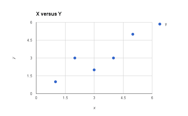
Plot of the Dataset for Simple Linear Regression

We can see the relationship between x and y looks kind-of linear. As in, we could probably draw a line somewhere diagonally from the bottom left of the plot to the top right to generally describe the relationship between the data. This is a good indication that using linear regression might be appropriate for this little dataset.

Get your FREE Algorithms Mind Map

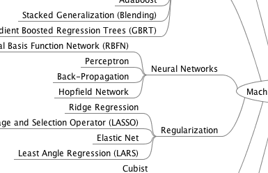
Sample of the handy machine learning algorithms mind map.

I've created a handy mind map of 60+ algorithms organized by type.

Download it, print it and use it. 

Simple Linear Regression

When we have a single in put attribute (x) and we want to use linear regression, this is called simple linear regression.

With simple linear regression we want to model our data as follows:

y = B0 + B1 * x

This is a line where y is the output variable we want to predict, x is the input variable we know and B0 and B1 are coefficients we need to estimate.

B0 is called the intercept because it determines where the line intercepts the y axis. In machine learning we can call this the bias, because it is added to offset all predictions that we make. The B1 term is called the slope because it defines the slope of the line or how x translates into a y value before we add our bias.

The model is called Simple Linear Regression because there is only one input variable (x). If there were more input variables (e.g. x1, x2, etc.) then this would be called multiple regression.

Stochastic Gradient Descent

Gradient Descent is the process of minimizing a function by following the gradients of the cost function.

This involves knowing the form of the cost as well as the derivative so that from a given point you know the gradient and can move in that direction, e.g. downhill towards the minimum value.

In Machine learning we can use a similar technique called stochastic gradient descent to minimize the error of a model on our training data.

The way this works is that each training instance is shown to the model one at a time. The model makes a prediction for a training instance, the error is calculated and the model is updated in order to reduce the error for the next prediction.

This procedure can be used to find the set of coefficients in a model that result in the smallest error for the model on the training data. Each iteration the coefficients, called weights (w) in machine learning language are updated using the equation:

w = w – alpha * delta

Where w is the coefficient or weight being optimized, alpha is a learning rate that you must configure (e.g. 0.1) and gradient is the error for the model on the training data attributed to the weight.

Simple Linear Regression with Stochastic Gradient Descent

The coefficients used in simple linear regression can be found using stochastic gradient descent.

Linear regression is a linear system and the coefficients can be calculated analytically using linear algebra. Stochastic gradient descent is not used to calculate the coefficients for linear regression in practice (in most cases).

Linear regression does provide a useful exercise for learning stochastic gradient descent which is an important algorithm used for minimizing cost functions by machine learning algorithms.

As stated above, our linear regression model is defined as follows:

y = B0 + B1 * x

Gradient Descent Iteration #1

Let’s start with values of 0.0 for both coefficients.

B0 = 0.0

B1 = 0.0

y = 0.0 + 0.0 * x

We can calculate the error for a prediction as follows:

error = p(i) – y(i)

Where p(i) is the prediction for the i’th instance in our dataset and y(i) is the i’th output variable for the instance in the dataset.

We can now calculate he predicted value for y using our starting point coefficients for the first training instance:

x=1, y=1

p(i) = 0.0 + 0.0 * 1

p(i) = 0

Using the predicted output, we can calculate our error:

error = 0 – 1

error = -1

We can now use this error in our equation for gradient descent to update the weights. We will start with updating the intercept first, because it is easier.

We can say that B0 is accountable for all of the error. This is to say that updating the weight will use just the error as the gradient. We can calculate the update for the B0 coefficient as follows:

B0(t+1) = B0(t) – alpha * error

Where B0(t+1) is the updated version of the coefficient we will use on the next training instance, B0(t) is the current value for B0 alpha is our learning rate and error is the error we calculate for the training instance. Let’s use a small learning rate of 0.01 and plug the values into the equation to work out what the new and slightly optimized value of B0 will be:

B0(t+1) = 0.0 – 0.01 * -1.0

B0(t+1) = 0.01

Now, let’s look at updating the value for B1. We use the same equation with one small change. The error is filtered by the input that caused it. We can update B1 using the equation:

B1(t+1) = B1(t) – alpha * error * x

Where B1(t+1) is the update coefficient, B1(t) is the current version of the coefficient, alpha is the same learning rate described above, error is the same error calculated above and x is the input value.

We can plug in our numbers into the equation and calculate the updated value for B1:

B1(t+1) = 0.0 – 0.01 * -1 * 1

B1(t+1) = 0.01

We have just finished the first iteration of gradient descent and we have updated our weights to be B0=0.01 and B1=0.01. This process must be repeated for the remaining 4 instances from our dataset.

One pass through the training dataset is called an epoch.

Gradient Descent Iteration #20

Let’s jump ahead.

You can repeat this process another 19 times. This is 4 complete epochs of the training data being exposed to the model and updating the coefficients.

Here is a list of all of the values for the coefficients over the 20 iterations that you should see:

I think that 20 iterations or 4 epochs is a nice round number and a good place to stop. You could keep going if you wanted.

Your values should match closely, but may have minor differences due to different spreadsheet programs and different precisions. You can plug each pair of coefficients back into the simple linear regression equation. This is useful because we can calculate a prediction for each training instance and in turn calculate the error.

Below is a plot of the error for each set of coefficients as the learning process unfolded. This is a useful graph as it shows us that error was decreasing with each iteration and starting to bounce around a bit towards the end.

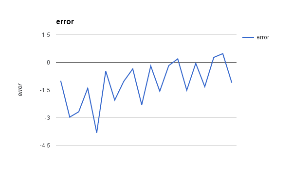
Linear Regression Gradient Descent Error versus Iteration

You can see that our final coefficients have the values B0=0.230897491 and B1=0.7904386102

Let’s plug them into our simple linear Regression model and make a prediction for each point in our training dataset.

We can plot our dataset again with these predictions overlaid (x vs y and x vs prediction). Drawing a line through the 5 predictions gives us an idea of how well the model fits the training data.

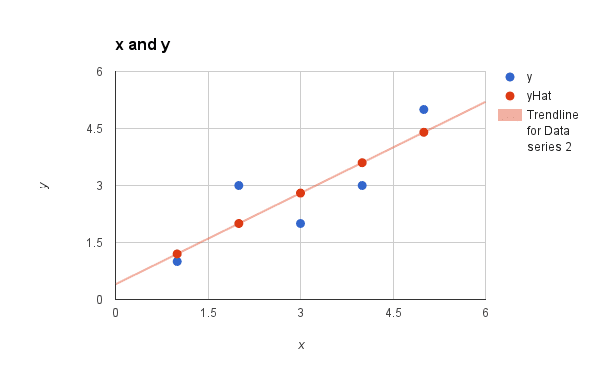
Simple Linear Regression Model

Summary

In this post you discovered the simple linear regression model and how to train it using stochastic gradient descent.

You work through the application of the update rule for gradient descent. You also learned how to make predictions with a learned linear regression model.

Do you have any questions about this post or about simple linear regression with stochastic gradient descent? Leave a comment and ask your question and I will do my best to answer it.

Discover How Machine Learning Algorithms Work!

See How Algorithms Work in Minutes

...with just arithmetic and simple examples

Discover how in my new Ebook:
Master Machine Learning Algorithms

It covers explanations and examples of 10 top algorithms, like:
Linear Regression, k-Nearest Neighbors, Support Vector Machines and much more...

Finally, Pull Back the Curtain on
Machine Learning Algorithms

Skip the Academics. Just Results.

See What's Inside