Exponential smoothing is a time series forecasting method for univariate data that can be extended to support data with a systematic trend or seasonal component.
It is common practice to use an optimization process to find the model hyperparameters that result in the exponential smoothing model with the best performance for a given time series dataset. This practice applies only to the coefficients used by the model to describe the exponential structure of the level, trend, and seasonality.
It is also possible to automatically optimize other hyperparameters of an exponential smoothing model, such as whether or not to model the trend and seasonal component and if so, whether to model them using an additive or multiplicative method.
In this tutorial, you will discover how to develop a framework for grid searching all of the exponential smoothing model hyperparameters for univariate time series forecasting.
After completing this tutorial, you will know:
How to develop a framework for grid searching ETS models from scratch using walk-forward validation.
How to grid search ETS model hyperparameters for daily time series data for female births.
How to grid search ETS model hyperparameters for monthly time series data for shampoo sales, car sales, and temperature.
Kick-start your project with my new book Deep Learning for Time Series Forecasting, including step-by-step tutorials and the Python source code files for all examples.
Let’s get started.
Updated Oc/2018: Updated fitting of ETS models to use NumPy array to fixes issues with multiplicative trend/seasonality (thanks Amit Amola).
Updated Apr/2019: Updated the link to dataset.
How to Grid Search Triple Exponential Smoothing for Time Series Forecasting in Python Photo by john mcsporran, some rights reserved.
Tutorial Overview
This tutorial is divided into six parts; they are:
Time series methods like the Box-Jenkins ARIMA family of methods develop a model where the prediction is a weighted linear sum of recent past observations or lags.
Exponential smoothing forecasting methods are similar in that a prediction is a weighted sum of past observations, but the model explicitly uses an exponentially decreasing weight for past observations.
Specifically, past observations are weighted with a geometrically decreasing ratio.
Forecasts produced using exponential smoothing methods are weighted averages of past observations, with the weights decaying exponentially as the observations get older. In other words, the more recent the observation, the higher the associated weight.
Exponential smoothing methods may be considered as peers and an alternative to the popular Box-Jenkins ARIMA class of methods for time series forecasting.
Collectively, the methods are sometimes referred to as ETS models, referring to the explicit modeling of Error, Trend, and Seasonality.
There are three types of exponential smoothing; they are:
Single Exponential Smoothing, or SES, for univariate data without trend or seasonality.
Double Exponential Smoothing for univariate data with support for trends.
Triple Exponential Smoothing, or Holt-Winters Exponential Smoothing, with support for both trends and seasonality.
A triple exponential smoothing model subsumes single and double exponential smoothing by the configuration of the nature of the trend (additive, multiplicative, or none) and the nature of the seasonality (additive, multiplicative, or none), as well as any dampening of the trend.
Need help with Deep Learning for Time Series?
Take my free 7-day email crash course now (with sample code).
Click to sign-up and also get a free PDF Ebook version of the course.
Develop a Grid Search Framework
In this section, we will develop a framework for grid searching exponential smoothing model hyperparameters for a given univariate time series forecasting problem.
This model has hyperparameters that control the nature of the exponential performed for the series, trend, and seasonality, specifically:
smoothing_level (alpha): the smoothing coefficient for the level.
smoothing_slope (beta): the smoothing coefficient for the trend.
smoothing_seasonal (gamma): the smoothing coefficient for the seasonal component.
damping_slope (phi): the coefficient for the damped trend.
All four of these hyperparameters can be specified when defining the model. If they are not specified, the library will automatically tune the model and find the optimal values for these hyperparameters (e.g. optimized=True).
There are other hyperparameters that the model will not automatically tune that you may want to specify; they are:
trend: The type of trend component, as either “add” for additive or “mul” for multiplicative. Modeling the trend can be disabled by setting it to None.
damped: Whether or not the trend component should be damped, either True or False.
seasonal: The type of seasonal component, as either “add” for additive or “mul” for multiplicative. Modeling the seasonal component can be disabled by setting it to None.
seasonal_periods: The number of time steps in a seasonal period, e.g. 12 for 12 months in a yearly seasonal structure.
use_boxcox: Whether or not to perform a power transform of the series (True/False) or specify the lambda for the transform.
If you know enough about your problem to specify one or more of these parameters, then you should specify them. If not, you can try grid searching these parameters.
We can start-off by defining a function that will fit a model with a given configuration and make a one-step forecast.
The exp_smoothing_forecast() below implements this behavior.
The function takes an array or list of contiguous prior observations and a list of configuration parameters used to configure the model.
The configuration parameters in order are: the trend type, the dampening type, the seasonality type, the seasonal period, whether or not to use a Box-Cox transform, and whether or not to remove the bias when fitting the model.
Next, we need to build up some functions for fitting and evaluating a model repeatedly via walk-forward validation, including splitting a dataset into train and test sets and evaluating one-step forecasts.
We can split a list or NumPy array of data using a slice given a specified size of the split, e.g. the number of time steps to use from the data in the test set.
The train_test_split() function below implements this for a provided dataset and a specified number of time steps to use in the test set.
1
2
3
# split a univariate dataset into train/test sets
def train_test_split(data,n_test):
returndata[:-n_test],data[-n_test:]
After forecasts have been made for each step in the test dataset, they need to be compared to the test set in order to calculate an error score.
There are many popular errors scores for time series forecasting. In this case, we will use root mean squared error (RMSE), but you can change this to your preferred measure, e.g. MAPE, MAE, etc.
The measure_rmse() function below will calculate the RMSE given a list of actual (the test set) and predicted values.
1
2
3
# root mean squared error or rmse
def measure_rmse(actual,predicted):
returnsqrt(mean_squared_error(actual,predicted))
We can now implement the walk-forward validation scheme. This is a standard approach to evaluating a time series forecasting model that respects the temporal ordering of observations.
First, a provided univariate time series dataset is split into train and test sets using the train_test_split() function. Then the number of observations in the test set are enumerated. For each, we fit a model on all of the history and make a one step forecast. The true observation for the time step is then added to the history, and the process is repeated. The exp_smoothing_forecast() function is called in order to fit a model and make a prediction. Finally, an error score is calculated by comparing all one-step forecasts to the actual test set by calling the measure_rmse() function.
The walk_forward_validation() function below implements this, taking a univariate time series, a number of time steps to use in the test set, and an array of model configurations.
1
2
3
4
5
6
7
8
9
10
11
12
13
14
15
16
17
18
# walk-forward validation for univariate data
def walk_forward_validation(data,n_test,cfg):
predictions=list()
# split dataset
train,test=train_test_split(data,n_test)
# seed history with training dataset
history=[xforxintrain]
# step over each time-step in the test set
foriinrange(len(test)):
# fit model and make forecast for history
yhat=exp_smoothing_forecast(history,cfg)
# store forecast in list of predictions
predictions.append(yhat)
# add actual observation to history for the next loop
history.append(test[i])
# estimate prediction error
error=measure_rmse(test,predictions)
returnerror
If you are interested in making multi-step predictions, you can change the call to predict() in the exp_smoothing_forecast() function and also change the calculation of error in the measure_rmse() function.
We can call walk_forward_validation() repeatedly with different lists of model configurations.
One possible issue is that some combinations of model configurations may not be called for the model and will throw an exception, e.g. specifying some but not all aspects of the seasonal structure in the data.
Further, some models may also raise warnings on some data, e.g. from the linear algebra libraries called by the statsmodels library.
We can trap exceptions and ignore warnings during the grid search by wrapping all calls to walk_forward_validation() with a try-except and a block to ignore warnings. We can also add debugging support to disable these protections in case we want to see what is really going on. Finally, if an error does occur, we can return a None result; otherwise, we can print some information about the skill of each model evaluated. This is helpful when a large number of models are evaluated.
The score_model() function below implements this and returns a tuple of (key and result), where the key is a string version of the tested model configuration.
1
2
3
4
5
6
7
8
9
10
11
12
13
14
15
16
17
18
19
20
21
# score a model, return None on failure
def score_model(data,n_test,cfg,debug=False):
result=None
# convert config to a key
key=str(cfg)
# show all warnings and fail on exception if debugging
ifdebug:
result=walk_forward_validation(data,n_test,cfg)
else:
# one failure during model validation suggests an unstable config
try:
# never show warnings when grid searching, too noisy
with catch_warnings():
filterwarnings("ignore")
result=walk_forward_validation(data,n_test,cfg)
except:
error=None
# check for an interesting result
ifresult isnotNone:
print(' > Model[%s] %.3f'%(key,result))
return(key,result)
Next, we need a loop to test a list of different model configurations.
This is the main function that drives the grid search process and will call the score_model() function for each model configuration.
We can dramatically speed up the grid search process by evaluating model configurations in parallel. One way to do that is to use the Joblib library.
We can define a Parallel object with the number of cores to use and set it to the number of CPU cores detected in your hardware.
The result of evaluating a list of configurations will be a list of tuples, each with a name that summarizes a specific model configuration and the error of the model evaluated with that configuration as either the RMSE or None if there was an error.
We can filter out all scores with a None.
1
scores=[rforrinscores ifr[1]!=None]
We can then sort all tuples in the list by the score in ascending order (best are first), then return this list of scores for review.
The grid_search() function below implements this behavior given a univariate time series dataset, a list of model configurations (list of lists), and the number of time steps to use in the test set. An optional parallel argument allows the evaluation of models across all cores to be tuned on or off, and is on by default.
The only thing left to do is to define a list of model configurations to try for a dataset.
We can define this generically. The only parameter we may want to specify is the periodicity of the seasonal component in the series, if one exists. By default, we will assume no seasonal component.
The exp_smoothing_configs() function below will create a list of model configurations to evaluate.
An optional list of seasonal periods can be specified, and you could even change the function to specify other elements that you may know about your time series.
In theory, there are 72 possible model configurations to evaluate, but in practice, many will not be valid and will result in an error that we will trap and ignore.
1
2
3
4
5
6
7
8
9
10
11
12
13
14
15
16
17
18
19
20
# create a set of exponential smoothing configs to try
def exp_smoothing_configs(seasonal=[None]):
models=list()
# define config lists
t_params=['add','mul',None]
d_params=[True,False]
s_params=['add','mul',None]
p_params=seasonal
b_params=[True,False]
r_params=[True,False]
# create config instances
fortint_params:
fordind_params:
forsins_params:
forpinp_params:
forbinb_params:
forrinr_params:
cfg=[t,d,s,p,b,r]
models.append(cfg)
returnmodels
We now have a framework for grid searching triple exponential smoothing model hyperparameters via one-step walk-forward validation.
It is generic and will work for any in-memory univariate time series provided as a list or NumPy array.
We can make sure all the pieces work together by testing it on a contrived 10-step dataset.
The complete example is listed below.
1
2
3
4
5
6
7
8
9
10
11
12
13
14
15
16
17
18
19
20
21
22
23
24
25
26
27
28
29
30
31
32
33
34
35
36
37
38
39
40
41
42
43
44
45
46
47
48
49
50
51
52
53
54
55
56
57
58
59
60
61
62
63
64
65
66
67
68
69
70
71
72
73
74
75
76
77
78
79
80
81
82
83
84
85
86
87
88
89
90
91
92
93
94
95
96
97
98
99
100
101
102
103
104
105
106
107
108
109
110
111
112
113
114
115
116
117
118
119
120
121
122
123
# grid search holt winter's exponential smoothing
from math import sqrt
from multiprocessing import cpu_count
from joblib import Parallel
from joblib import delayed
from warnings import catch_warnings
from warnings import filterwarnings
from statsmodels.tsa.holtwinters import ExponentialSmoothing
We do not report the model parameters optimized by the model itself. It is assumed that you can achieve the same result again by specifying the broader hyperparameters and allow the library to find the same internal parameters.
You can access these internal parameters by refitting a standalone model with the same configuration and printing the contents of the ‘params‘ attribute on the model fit; for example:
1
print(model_fit.params)
Now that we have a robust framework for grid searching ETS model hyperparameters, let’s test it out on a suite of standard univariate time series datasets.
The datasets were chosen for demonstration purposes; I am not suggesting that an ETS model is the best approach for each dataset, and perhaps an SARIMA or something else would be more appropriate in some cases.
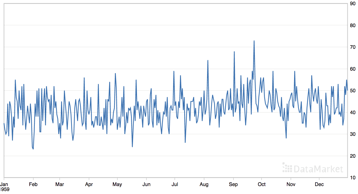
Case Study 1: No Trend or Seasonality
The ‘daily female births’ dataset summarizes the daily total female births in California, USA in 1959.
The dataset has no obvious trend or seasonal component.
Running the example may take a few minutes as fitting each ETS model can take about a minute on modern hardware.
Model configurations and the RMSE are printed as the models are evaluated The top three model configurations and their error are reported at the end of the run.
Note: Your results may vary given the stochastic nature of the algorithm or evaluation procedure, or differences in numerical precision. Consider running the example a few times and compare the average outcome.
We can see that the best result was an RMSE of about 6.96 births with the following configuration:
Trend: Multiplicative
Damped: False
Seasonal: None
Seasonal Periods: None
Box-Cox Transform: True
Remove Bias: True
What is surprising is that a model that assumed an multiplicative trend performed better than one that didn’t.
We would not know that this is the case unless we threw out assumptions and grid searched models.
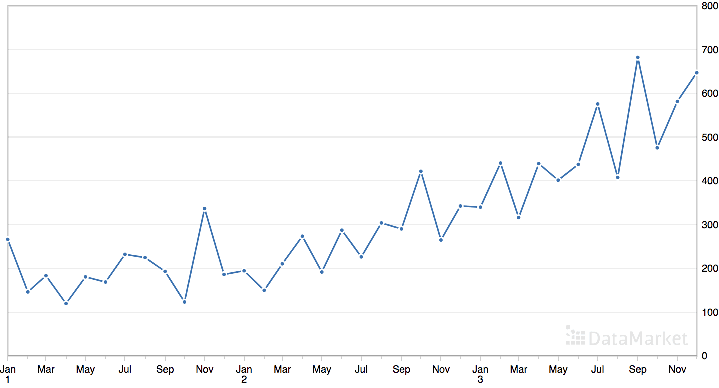
Running the example is fast given there are a small number of observations.
Model configurations and the RMSE are printed as the models are evaluated. The top three model configurations and their error are reported at the end of the run.
Note: Your results may vary given the stochastic nature of the algorithm or evaluation procedure, or differences in numerical precision. Consider running the example a few times and compare the average outcome.
We can see that the best result was an RMSE of about 83.74 sales with the following configuration:
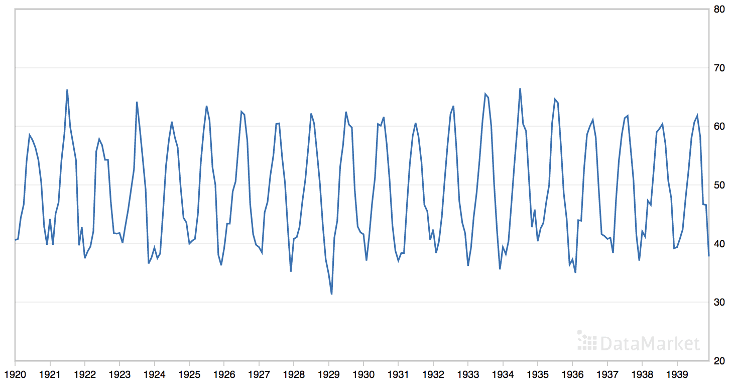
The ‘monthly mean temperatures’ dataset summarizes the monthly average air temperatures in Nottingham Castle, England from 1920 to 1939 in degrees Fahrenheit.
The dataset has an obvious seasonal component and no obvious trend.
Line Plot of the Monthly Mean Temperatures Dataset
We will trim the dataset to the last five years of data (60 observations) in order to speed up the model evaluation process and use the last year, or 12 observations, for the test set.
1
2
# trim dataset to 5 years
data=data[-(5*12):]
The period of the seasonal component is about one year, or 12 observations.
We will use this as the seasonal period in the call to the exp_smoothing_configs() function when preparing the model configurations.
1
2
# model configs
cfg_list=exp_smoothing_configs(seasonal=[0,12])
The complete example grid searching the monthly mean temperature time series forecasting problem is listed below.
1
2
3
4
5
6
7
8
9
10
11
12
13
14
15
16
17
18
19
20
21
22
23
24
25
26
27
28
29
30
31
32
33
34
35
36
37
38
39
40
41
42
43
44
45
46
47
48
49
50
51
52
53
54
55
56
57
58
59
60
61
62
63
64
65
66
67
68
69
70
71
72
73
74
75
76
77
78
79
80
81
82
83
84
85
86
87
88
89
90
91
92
93
94
95
96
97
98
99
100
101
102
103
104
105
106
107
108
109
110
111
112
113
114
115
116
117
118
119
120
121
122
123
124
125
126
# grid search ets hyperparameters for monthly mean temp dataset
from math import sqrt
from multiprocessing import cpu_count
from joblib import Parallel
from joblib import delayed
from warnings import catch_warnings
from warnings import filterwarnings
from statsmodels.tsa.holtwinters import ExponentialSmoothing
Running the example is relatively slow given the large amount of data.
Model configurations and the RMSE are printed as the models are evaluated. The top three model configurations and their error are reported at the end of the run.
Note: Your results may vary given the stochastic nature of the algorithm or evaluation procedure, or differences in numerical precision. Consider running the example a few times and compare the average outcome.
We can see that the best result was an RMSE of about 1.50 degrees with the following configuration:
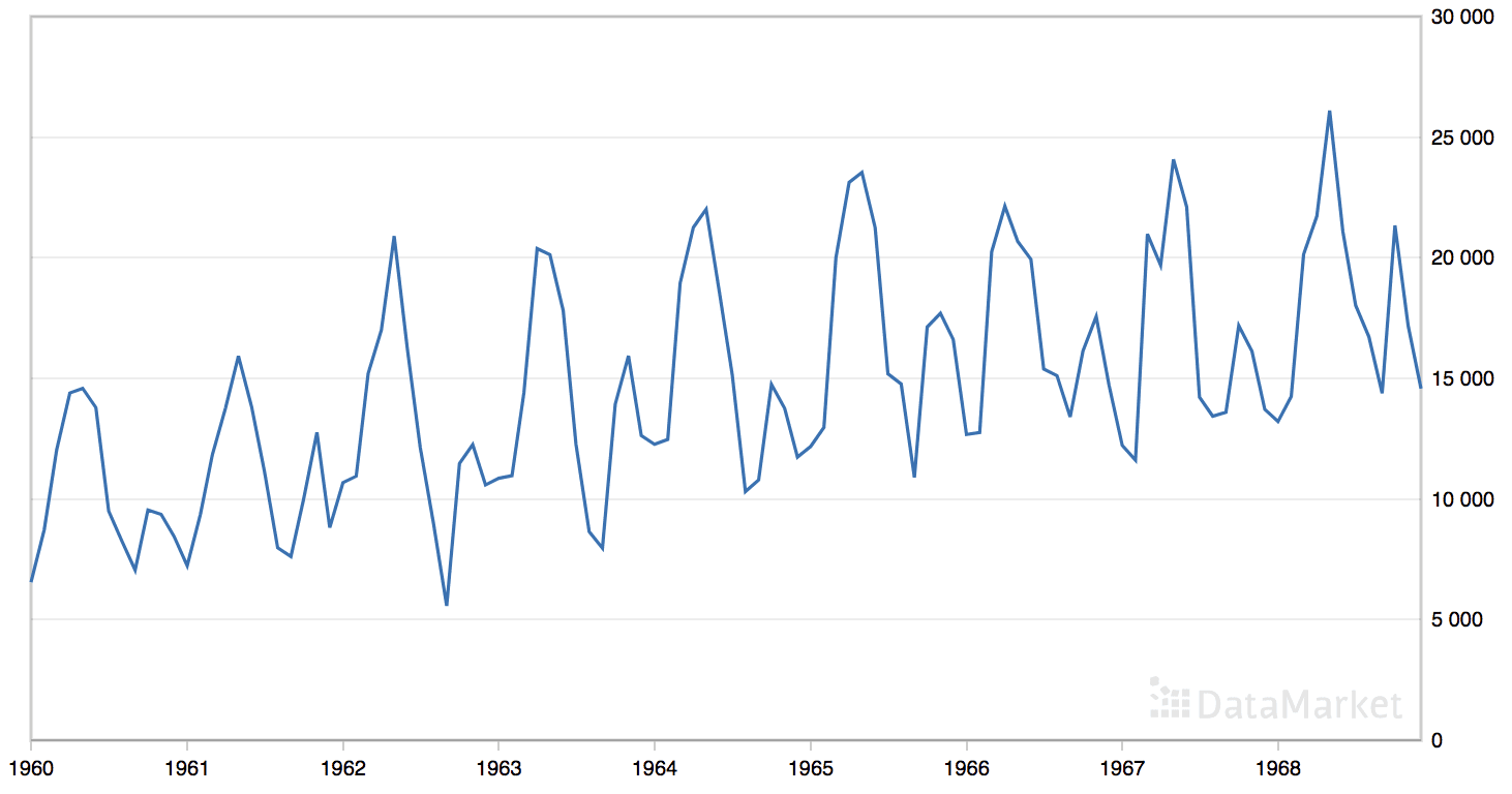
The dataset has nine years, or 108 observations. We will use the last year, or 12 observations, as the test set.
The period of the seasonal component could be six months or 12 months. We will try both as the seasonal period in the call to the exp_smoothing_configs() function when preparing the model configurations.
1
2
# model configs
cfg_list=exp_smoothing_configs(seasonal=[0,6,12])
The complete example grid searching the monthly car sales time series forecasting problem is listed below.
1
2
3
4
5
6
7
8
9
10
11
12
13
14
15
16
17
18
19
20
21
22
23
24
25
26
27
28
29
30
31
32
33
34
35
36
37
38
39
40
41
42
43
44
45
46
47
48
49
50
51
52
53
54
55
56
57
58
59
60
61
62
63
64
65
66
67
68
69
70
71
72
73
74
75
76
77
78
79
80
81
82
83
84
85
86
87
88
89
90
91
92
93
94
95
96
97
98
99
100
101
102
103
104
105
106
107
108
109
110
111
112
113
114
115
116
117
118
119
120
121
122
123
124
# grid search ets models for monthly car sales
from math import sqrt
from multiprocessing import cpu_count
from joblib import Parallel
from joblib import delayed
from warnings import catch_warnings
from warnings import filterwarnings
from statsmodels.tsa.holtwinters import ExponentialSmoothing
Running the example is slow given the large amount of data.
Model configurations and the RMSE are printed as the models are evaluated. The top three model configurations and their error are reported at the end of the run.
Note: Your results may vary given the stochastic nature of the algorithm or evaluation procedure, or differences in numerical precision. Consider running the example a few times and compare the average outcome.
We can see that the best result was an RMSE of about 1,672 sales with the following configuration:
Trend: Additive
Damped: False
Seasonal: Additive
Seasonal Periods: 12
Box-Cox Transform: False
Remove Bias: True
This is a little surprising as I would have guessed that a six-month seasonal model would be the preferred approach.
This section lists some ideas for extending the tutorial that you may wish to explore.
Data Transforms. Update the framework to support configurable data transforms such as normalization and standardization.
Plot Forecast. Update the framework to re-fit a model with the best configuration and forecast the entire test dataset, then plot the forecast compared to the actual observations in the test set.
Tune Amount of History. Update the framework to tune the amount of historical data used to fit the model (e.g. in the case of the 10 years of max temperature data).
If you explore any of these extensions, I’d love to know.
Further Reading
This section provides more resources on the topic if you are looking to go deeper.
In this tutorial, you discovered how to develop a framework for grid searching all of the exponential smoothing model hyperparameters for univariate time series forecasting.
Specifically, you learned:
How to develop a framework for grid searching ETS models from scratch using walk-forward validation.
How to grid search ETS model hyperparameters for daily time series data for births.
How to grid search ETS model hyperparameters for monthly time series data for shampoo sales, car sales and temperature.
Do you have any questions?
Ask your questions in the comments below and I will do my best to answer.
Develop Deep Learning models for Time Series Today!
=>sorry,dear.my nam… Jon. Living now “Bangladesh” proffsanally me 15yeasr my life supot my brothers business said, mobilephone service and seal said,so technology said allows real us so good,bat i am not Happy because i no job, only miss us moneys, so one qus???
=>god son for you,any good said us me,and my barind,?give me you my life.
=>one help full job, (i no interst job service moneys/only free service? Your couasc god son any poor man)us me?pleasc dear,
@-joni
Hey Jason,
So I tried this above code, but one interesting issue that’s occurring is that it is not performing the ETS on whenever there is multiplicative trend or seasonality. If you see your results as well, you’ll notice this thing.
Since you are using try and except, this isn’t giving an error, but in the actual case, it gives error by saying that endog<=0.0
Now with a 0 value in the TS data, this analogy makes sense, but even your dataset cases, there is no 0 value as such. So why is it happening and can you just check if that's what happening in your case as well.
Moreover, I converted my time series data into just an array of values and this worked. But the same thing you have done but it still doesn't give any multiplicative results in your code that you've created. Can you take a look.
You’re right. I have updated the usage of the ExponentialSmoothing to take a numpy array instead of a list. This results in correct usage of ‘mul’ for trend and seasonality.
This code either does not work for me, or takes a very very long time to run (I do not get an error). My dataset only has 25 time points. The last block of code looks like this:
Perhaps try fewer configurations?
Perhaps try running over night?
Perhaps try running on a larger machine (ec2 instance)?
Perhaps try running on less data?
I have created an OOP version of the above code. But when Parallel is set to True, it gives following error:
File “models.py”, line 190, in //models.py is my file
param = wh.grid_search(parallel=True)
File models.py”, line 104, in grid_search
self.scores = executor(tasks)
File .conda/envs/python3.6/lib/python3.6/site-packages/joblib/parallel.py”, line 934, in __call__
self.retrieve()
File .conda/envs/python3.6/lib/python3.6/site-packages/joblib/parallel.py”, line 833, in retrieve
self._output.extend(job.get(timeout=self.timeout))
File .conda/envs/python3.6/lib/python3.6/multiprocessing/pool.py”, line 644, in get
raise self._value
File .conda/envs/python3.6/lib/python3.6/multiprocessing/pool.py”, line 424, in _handle_tasks
put(task)
File .conda/envs/python3.6/lib/python3.6/site-packages/joblib/pool.py”, line 158, in send
CustomizablePickler(buffer, self._reducers).dump(obj)
File “.conda/envs/python3.6/lib/python3.6/site-packages/statsmodels/graphics/functional.py”, line 32, in _pickle_method
if m.im_self is None:
AttributeError: ‘function’ object has no
attribute ‘im_self’
Very, very well done Jason. I am impressed by your concise code and smart implementation of parallel processing. I do have a comment and a request that might be useful to others that look at these well-done case studies.
First I believe that “…all cores to be tuned on …” should be replaced by “…all cores to be turned on…”
Second, could you expand on “multi-step predictions”. More specifically, show code that could be used to actually do this and to perform “multi-step predictions” beyond the data that you actually have.
Also, I did need to add the following first line statement to all of your examples:
# coding:utf-8
Otherwise, an exception is thrown, and the code will not execute.
first of all, thank you very much for the knowledge and code you share with all of us! I am well into reading my second book from your forecasting series and struggling a bit with multi step ETS forecasting.
What I want to do is, I want to optimize the best ETS model and its hyperparameters for a 6 month prediction into the future. I imagine I would have to change the measure_rmse function so that it will be able to calculate the average error rate over 6 months and accordingly change its hyperparameters to minimize this error rate. I was thinking about creating a sum of the RMSEs and dividing this by the amount of months, i.e. 6 months.
However, I can’t get it working. I based the function on the evaluate_forecasts function from the multi step ARIMA forecasting part in your book “deep learning for time series forecasting”. Could you help me out and provide me with an example on how I should change the measure_rmse function to optimize for an ETS model 6 months into the future.
Very informative article, thanks! I have the following two questions:
1) I have multiple time series to forecast daily (e.g. forecast the demand for products). The time period (date of first data point – date of last data point) of the time series is not fixed, which may vary from 2 years (~730) data points, or even 2 months (~60 data points). How do I decide the seasonal parameters in these 2 different scenarios?
2) My time series will have zeros in it. Practically, a product cannot have a demand daily, but the output I want is a daily demand (with checking the seasonality). So I will need to add the missing dates in the time series and add zeros (zero demand) for the missing dates. How can I best leverage this algorithm for the following scenario?
Thanks for your reply. What I mean by the seasonal parameter is, should it be 365 for daily? or 12 or 0? I didn’t understand how the seasonal parameter is exactly set. Thanks for the smoothing suggestion!
I am having one basic question. Once we find the optimal parameters and fit the data into mode al and moving to prediction.
1.ex i am converting non stationary input to stationary by using log or decompose and feeding.
So when i feed that stationary data into model fit and predict. the model will predict based on the stationary data? or it will directly return the final numbers?
2.if it just return based on stationary data, how i can convert into proper numbers? ex i have used decompose method and taken residual to model fit and prediction
thank you for your post. I try to refit the model with the bests configuration from the grid search. As data I pass the whole dataset (no test/training split). With the “optimal” configuration I get the error:
ConvergenceWarning: Optimization failed to converge. Check mle_retvals. ConvergenceWarning).
With the “third-best” config it converges. Any idea why that might be? Shouldn’t it work with all scored configs?
I use the config returned by the grid search. I also tried to fit the model just with the training data – it also fails to converge. My guess is, that since warnings are supressed in the grid search it fails to converge during the scoring as well. Are models that do not converge added to the score?
Hello Jason
When I run your code above with the # define dataset
data = [10.0, 20.0, 30.0, 40.0, 50.0, 60.0, 70.0, 80.0, 90.0, 100.0]
then I get an AttributeError: Can’t get Attribute ‘score_model’ on . What is wrong?
Thank you very much for your help.
Best regards
Peter
Traceback (most recent call last):
File “C:\ProgramData\Anaconda-2018.12\lib\multiprocessing\process.py”, line 297, in _bootstrap
self.run()
File “C:\ProgramData\Anaconda-2018.12\lib\multiprocessing\process.py”, line 99, in run
self._target(*self._args, **self._kwargs)
File “C:\ProgramData\Anaconda-2018.12\lib\multiprocessing\pool.py”, line 110, in worker
task = get()
File “C:\ProgramData\Anaconda-2018.12\lib\site-packages\joblib\pool.py”, line 149, in get
return recv()
File “C:\ProgramData\Anaconda-2018.12\lib\multiprocessing\connection.py”, line 251, in recv
return _ForkingPickler.loads(buf.getbuffer())
AttributeError: Can’t get attribute ‘score_model’ on
Jason – thanks for your great post.
Q1:I have been trying to replicate your results for last 3 days, without luck. Not sure whats the problem. I think there is something incorrect in your code, and I don’t say that lightly and respect what you have done. I truly hope I am wrong but after spending 3 days, I could not reproduce any of your rmse values.
Just take the car sales example. Your code shows the lowest rmse (1672) for [‘add’, False, ‘add’, 12, False, True] combination. If I fit the model using those exact same params, I get 1664. That may look trivial but the difference is hige for other values. If I take [‘add’, True, ‘add’, 6, False, True] combination, you got 3240 and I got 6487.
It was the same case all other examples in this post. Are you able to reproduce your values if you enter the parameters individually? I am not sure whats causing it. see the code below.
Q2: If I calculate the rmse for test set and also AIC, shouldnt we be using the parameters that have the lowest AIC since it approximate cross-validation? In some case in above examples, the parameters that had lowest test_rmse didnt necessarily have lowest AIC. what approach would you suggest?
Thanks for your great posts.
import pandas as pd
import numpy as np
import itertools
from statsmodels.tsa.holtwinters import ExponentialSmoothing
from sklearn.metrics import mean_squared_error
Jason – Thanks a lot for such an informative article.
I have a doubt regarding use of similar implementation for forecasting of traffic. But for most configuration params, it results in warning:
/usr/local/lib/python3.6/dist-packages/statsmodels/tsa/holtwinters.py:712: ConvergenceWarning: Optimization failed to converge. Check mle_retvals.
ConvergenceWarning)
I am trying to reproduce the Case Study 1: daily female births by copying the data set daily-total-female-births.csv to my local.
The code is running forever and not producing any result.
Am I missing anything here?
Below is what I am running.
Code:
# grid search ets models for daily female births
from math import sqrt
from multiprocessing import cpu_count
from joblib import Parallel
from joblib import delayed
from warnings import catch_warnings
from warnings import filterwarnings
from statsmodels.tsa.holtwinters import ExponentialSmoothing
from sklearn.metrics import mean_squared_error
from pandas import read_csv
from numpy import array
# one-step Holt Winter’s Exponential Smoothing forecast
def exp_smoothing_forecast(history, config):
t,d,s,p,b,r = config
# define model
history = array(history)
model = ExponentialSmoothing(history, trend=t, damped=d, seasonal=s, seasonal_periods=p)
# fit model
model_fit = model.fit(optimized=True, use_boxcox=b, remove_bias=r)
# make one step forecast
yhat = model_fit.predict(len(history), len(history))
return yhat[0]
# root mean squared error or rmse
def measure_rmse(actual, predicted):
return sqrt(mean_squared_error(actual, predicted))
# split a univariate dataset into train/test sets
def train_test_split(data, n_test):
return data[:-n_test], data[-n_test:]
# walk-forward validation for univariate data
def walk_forward_validation(data, n_test, cfg):
predictions = list()
# split dataset
train, test = train_test_split(data, n_test)
# seed history with training dataset
history = [x for x in train]
# step over each time-step in the test set
for i in range(len(test)):
# fit model and make forecast for history
yhat = exp_smoothing_forecast(history, cfg)
# store forecast in list of predictions
predictions.append(yhat)
# add actual observation to history for the next loop
history.append(test[i])
# estimate prediction error
error = measure_rmse(test, predictions)
return error
# score a model, return None on failure
def score_model(data, n_test, cfg, debug=False):
result = None
# convert config to a key
key = str(cfg)
# show all warnings and fail on exception if debugging
if debug:
result = walk_forward_validation(data, n_test, cfg)
else:
# one failure during model validation suggests an unstable config
try:
# never show warnings when grid searching, too noisy
with catch_warnings():
filterwarnings(“ignore”)
result = walk_forward_validation(data, n_test, cfg)
except:
error = None
# check for an interesting result
if result is not None:
print(‘ > Model[%s] %.3f’ % (key, result))
return (key, result)
# grid search configs
def grid_search(data, cfg_list, n_test, parallel=True):
scores = None
if parallel:
# execute configs in parallel
executor = Parallel(n_jobs=cpu_count(), backend=’multiprocessing’)
tasks = (delayed(score_model)(data, n_test, cfg) for cfg in cfg_list)
scores = executor(tasks)
else:
scores = [score_model(data, n_test, cfg) for cfg in cfg_list]
# remove empty results
scores = [r for r in scores if r[1] != None]
# sort configs by error, asc
scores.sort(key=lambda tup: tup[1])
return scores
# create a set of exponential smoothing configs to try
def exp_smoothing_configs(seasonal=[None]):
models = list()
# define config lists
t_params = [‘add’, ‘mul’, None]
d_params = [True, False]
s_params = [‘add’, ‘mul’, None]
p_params = seasonal
b_params = [True, False]
r_params = [True, False]
# create config instances
for t in t_params:
for d in d_params:
for s in s_params:
for p in p_params:
for b in b_params:
for r in r_params:
cfg = [t,d,s,p,b,r]
models.append(cfg)
return models
if __name__ == ‘__main__’:
# load dataset
series = read_csv(‘daily-total-female-births.csv’, header=0, index_col=0)
data = series.values
# data split
n_test = 165
# model configs
cfg_list = exp_smoothing_configs()
# grid search
scores = grid_search(data[:,0], cfg_list, n_test)
print(‘done’)
# list top 3 configs
for cfg, error in scores[:3]:
print(cfg, error)
I am implementing your code, but it seems like running it without parallel is a lot faster than running it with parallel. The problem is that some of my grid searches take more tan an hour when running without parallel.
I am trying to make it faster. Do you have any idea of why parallel is no helping? I am running exactly your same code. The number of CPUs in my computer is 4.
This article seems to have helped me find a good fit for the data I am trying to generate a forecast on.
Does the “The Deep Learning for Time Series” have the tutorials to take the model that seems to fit and then show us how to apply that model to forecast values for a series of future time intervals or anything along those lines?
It is such a wonderful tutorial! I am a new to time series analysis, your tutorial clearly show the train steps and one-step prediction, which is really helpful!
Here I have a small question. After training and finally obtaining the best model, next time I need to predict in real time. Do I need to retrain each time when getting one new observation? It seems will be really time-consuming.
In machine learning classification, it is not necessary to retrain each time as we can reuse the previously fitted models to predict. It is based on the assumption that samples are i.i.d. But how to manage this in time series? Apparently, most time series data points are highly autocorrelated.
A good tutorial on parameter tuning for Exponential Smoothing .
In this method, we are attempting all the permutations of parameters .
I have a question on ‘seasonal_periods’ param.
If a time series does not have strong seasonality … for e.g where there is repeat in the spike or trough based on certain holidays . In this case , when we create different train and test date windows, the ‘seasonal_periods’ parameter will vary depending on the training data .
So then how do we change its value , based on visual inspection of train data ??
Hi Jason. Tried that . The RMSE was quite large by setting it to ‘None’ and also on visual inspection , the predictions weren’t following the spikes in the actual values .
The problem is observed when I shrink the train window.
Working on that.
Thanks .
Great article.
do you know if it there is any way to wrap statsmodel’s models in a sklearn pipeline.
i tried but it throws an error that last object should implement a fit() method.
I had to use pmdarima to solve my issue but since statsmodel has wider range of algorithms, do you know if there is any way to accomplish the same?
Hi Jason,
First of all thank you for great tutorial. The last data set you used with trend and seasonality, the optimum configuration suggested by the code is
Trend: Additive
Damped: False
Seasonal: Additive
Seasonal Periods: 12
Box-Cox Transform: False
Remove Bias: True
Now my question is how it is possible to remove bias without performing the box-cox transformation?
I am very new to this field and just learning and my understanding is if you perform the power transformation then while reversing the transformation there may be bias so to remove that we use remove bias but in this case the series is not transformed in first place so why we need to remove bias?
Forgive me if it is stupid question.
Excellent article and tutorial Jason. Thank you for sharing.
I posted this question on Stack Cross Validated — questions about how to forecast quarterly financial data (revenues, cash flows, etc.). I believe you’ve asnwered my question using your case study #4 with Trend and Seasonality. I do wonder if I need to transform my data np.log(data) before predicting first?
when i run the SHAMPOO example, and basically every other data set with trend and no seasonality
i always get a prediction that looks like a straight ascending linear line (which is of course not good).
i get the configuration from your code and then apply it on the predict and this is what happens… any ideas? does it make sense?
hello jason,
let me 1st say that you’re doing a great job, you’re code is working great. Still it returns just about a 3 configuration and not all the possible ones. Moreover, given certain set of data it didn’t return any results at all.
Can you please help me.
How do you create a model once the optimal parameters have been found? I’m not sure how to use the array of params for the best model from the scores array?
Thank you for sharing this post. It was really helpful. However, I encountered some issues with the parallel part and use_boxcox. I noticed that the code gives better results when we specify the alpha and beta values. Here’s the modified code that worked for me:
# grid search ets models for monthly car sales
from math import sqrt
from multiprocessing import cpu_count
from joblib import Parallel
from joblib import delayed
from warnings import catch_warnings
from warnings import filterwarnings
from statsmodels.tsa.holtwinters import ExponentialSmoothing
from sklearn.metrics import mean_squared_error
from pandas import read_csv
from numpy import array
# one-step Holt Winter’s Exponential Smoothing forecast
def exp_smoothing_forecast(history, config):
t,d,s,p,r,alpha,beta = config
# define model
history = array(history)
model = ExponentialSmoothing(history, trend=t, damped=d, seasonal=s, seasonal_periods=p)
# fit model
model_fit = model.fit(optimized=True,smoothing_level=alpha, smoothing_slope=beta, remove_bias=r)
# make one step forecast
yhat = model_fit.predict(len(history), len(history))
return yhat[0]
# root mean squared error or rmse
def measure_rmse(actual, predicted):
return sqrt(mean_squared_error(actual, predicted))
# split a univariate dataset into train/test sets
def train_test_split(data, n_test):
return data[:-n_test], data[-n_test:]
# walk-forward validation for univariate data
def walk_forward_validation(data, n_test, cfg):
predictions = list()
# split dataset
train, test = train_test_split(data, n_test)
# seed history with training dataset
history = [x for x in train]
# step over each time-step in the test set
for i in range(len(test)):
# fit model and make forecast for history
yhat = exp_smoothing_forecast(history, cfg)
# store forecast in list of predictions
predictions.append(yhat)
# add actual observation to history for the next loop
history.append(test[i])
# estimate prediction error
error = measure_rmse(test, predictions)
return error
# score a model, return None on failure
def score_model(data, n_test, cfg, debug=False):
result = None
# convert config to a key
key = str(cfg)
# show all warnings and fail on exception if debugging
if debug:
result = walk_forward_validation(data, n_test, cfg)
else:
# one failure during model validation suggests an unstable config
try:
# never show warnings when grid searching, too noisy
with catch_warnings():
filterwarnings(“ignore”)
result = walk_forward_validation(data, n_test, cfg)
except:
error = None
# check for an interesting result
if result is not None:
print(‘ > Model[%s] %.3f’ % (key, result))
return (key, result)
# grid search configs
def grid_search(data, cfg_list, n_test, parallel=False):
scores = None
if parallel:
# execute configs in parallel
executor = Parallel(n_jobs=cpu_count(), backend=’multiprocessing’)
tasks = (delayed(score_model)(data, n_test, cfg) for cfg in cfg_list)
scores = executor(tasks)
else:
scores = [score_model(data, n_test, cfg) for cfg in cfg_list]
# remove empty results
scores = [r for r in scores if r[1] != None]
# sort configs by error, asc
scores.sort(key=lambda tup: tup[1])
return scores
def exp_smoothing_configs(seasonal=[None]):
models = list()
# define config lists
t_params = [‘add’, ‘mul’, None]
d_params = [True, False]
s_params = [‘add’, ‘mul’, None]
p_params = seasonal
r_params = [True, False]
alpha_params = [0.2, 0.4, 0.6, 0.8]
beta_params = [0.2, 0.4, 0.6, 0.8]
# create config instances
for t in t_params:
for d in d_params:
for s in s_params:
for p in p_params:
for r in r_params:
for alpha in alpha_params:
for beta in beta_params:
cfg = [t,d,s,p,r,alpha,beta]
models.append(cfg)
return models
if __name__ == ‘__main__’:
# define dataset
data = read_csv( ‘./data’)
series = data[[‘var’]]
data = series.values
print(data)
# data split
n_test = 12
# model configs
# cfg_list = exp_smoothing_configs(seasonal=[0,25])
cfg_list = exp_smoothing_configs(seasonal=[25])
# grid search
scores = grid_search(data[:,0], cfg_list, n_test)
print(‘done’)
# list top 3 configs
for cfg, error in scores[:3]:
print(cfg, error)
I hope this helps anyone who might be facing the same issue. Thank you again for sharing this valuable post.


=>sorry,dear.my nam… Jon. Living now “Bangladesh” proffsanally me 15yeasr my life supot my brothers business said, mobilephone service and seal said,so technology said allows real us so good,bat i am not Happy because i no job, only miss us moneys, so one qus???
=>god son for you,any good said us me,and my barind,?give me you my life.
=>one help full job, (i no interst job service moneys/only free service? Your couasc god son any poor man)us me?pleasc dear,
@-joni
Sorry, I don’t follow.
Thanks a lot , very interesting article !!!
Thanks.
Hey Jason,
So I tried this above code, but one interesting issue that’s occurring is that it is not performing the ETS on whenever there is multiplicative trend or seasonality. If you see your results as well, you’ll notice this thing.
Since you are using try and except, this isn’t giving an error, but in the actual case, it gives error by saying that endog<=0.0
Now with a 0 value in the TS data, this analogy makes sense, but even your dataset cases, there is no 0 value as such. So why is it happening and can you just check if that's what happening in your case as well.
Moreover, I converted my time series data into just an array of values and this worked. But the same thing you have done but it still doesn't give any multiplicative results in your code that you've created. Can you take a look.
Thanks, I’ll investigate.
UPDATE
You’re right. I have updated the usage of the ExponentialSmoothing to take a numpy array instead of a list. This results in correct usage of ‘mul’ for trend and seasonality.
I have updated the code in all examples. Thanks!
This code either does not work for me, or takes a very very long time to run (I do not get an error). My dataset only has 25 time points. The last block of code looks like this:
Is there a reason for this?
Yes, unfortunately the codes no longer work. I copied this exact example on the same csv file, and the code does not run.
The example in the tutorial does work, but assumes all of your libraries are up to date and that you’re using Python 3.5+.
I have some suggestions:
Perhaps try fewer configurations?
Perhaps try running over night?
Perhaps try running on a larger machine (ec2 instance)?
Perhaps try running on less data?
I have created an OOP version of the above code. But when Parallel is set to True, it gives following error:
File “models.py”, line 190, in //models.py is my file
param = wh.grid_search(parallel=True)
File models.py”, line 104, in grid_search
self.scores = executor(tasks)
File .conda/envs/python3.6/lib/python3.6/site-packages/joblib/parallel.py”, line 934, in __call__
self.retrieve()
File .conda/envs/python3.6/lib/python3.6/site-packages/joblib/parallel.py”, line 833, in retrieve
self._output.extend(job.get(timeout=self.timeout))
File .conda/envs/python3.6/lib/python3.6/multiprocessing/pool.py”, line 644, in get
raise self._value
File .conda/envs/python3.6/lib/python3.6/multiprocessing/pool.py”, line 424, in _handle_tasks
put(task)
File .conda/envs/python3.6/lib/python3.6/site-packages/joblib/pool.py”, line 158, in send
CustomizablePickler(buffer, self._reducers).dump(obj)
File “.conda/envs/python3.6/lib/python3.6/site-packages/statsmodels/graphics/functional.py”, line 32, in _pickle_method
if m.im_self is None:
AttributeError: ‘function’ object has no
attribute ‘im_self’
Could you please investigate and help
Hey I have managed to overcome the error. It was due to the following import statement:
from pmdarima.arima import auto_arima
I’m happy to hear that.
Sorry, I have not seen this error.
Perhaps try searching/posting on stackoverflow?
Very, very well done Jason. I am impressed by your concise code and smart implementation of parallel processing. I do have a comment and a request that might be useful to others that look at these well-done case studies.
First I believe that “…all cores to be tuned on …” should be replaced by “…all cores to be turned on…”
Second, could you expand on “multi-step predictions”. More specifically, show code that could be used to actually do this and to perform “multi-step predictions” beyond the data that you actually have.
Also, I did need to add the following first line statement to all of your examples:
# coding:utf-8
Otherwise, an exception is thrown, and the code will not execute.
Congratulatios on this tutorial J.B. 🙂
Thanks.
The predict() function can take the range of dates or indexes you require to make a multi-step prediction.
Use indexes and experiment with a 2 step forecast first, e.g.:
Best Jason,
first of all, thank you very much for the knowledge and code you share with all of us! I am well into reading my second book from your forecasting series and struggling a bit with multi step ETS forecasting.
What I want to do is, I want to optimize the best ETS model and its hyperparameters for a 6 month prediction into the future. I imagine I would have to change the measure_rmse function so that it will be able to calculate the average error rate over 6 months and accordingly change its hyperparameters to minimize this error rate. I was thinking about creating a sum of the RMSEs and dividing this by the amount of months, i.e. 6 months.
However, I can’t get it working. I based the function on the evaluate_forecasts function from the multi step ARIMA forecasting part in your book “deep learning for time series forecasting”. Could you help me out and provide me with an example on how I should change the measure_rmse function to optimize for an ETS model 6 months into the future.
Thanks in advance!
Yes.
I know I have tutorials on the blog that evaluate RMSE for multi-step forecasts, perhaps you can adapt the code from one of them, such as:
https://machinelearningmastery.com/multi-step-time-series-forecasting-long-short-term-memory-networks-python/
Hi Jason,
Very informative article, thanks! I have the following two questions:
1) I have multiple time series to forecast daily (e.g. forecast the demand for products). The time period (date of first data point – date of last data point) of the time series is not fixed, which may vary from 2 years (~730) data points, or even 2 months (~60 data points). How do I decide the seasonal parameters in these 2 different scenarios?
2) My time series will have zeros in it. Practically, a product cannot have a demand daily, but the output I want is a daily demand (with checking the seasonality). So I will need to add the missing dates in the time series and add zeros (zero demand) for the missing dates. How can I best leverage this algorithm for the following scenario?
Thanks
Perhaps test different configurations in order to discover what works best?
Perhaps try smoothing the data prior to fitting the model to even out the zeros?
Hi Jason,
Thanks for your reply. What I mean by the seasonal parameter is, should it be 365 for daily? or 12 or 0? I didn’t understand how the seasonal parameter is exactly set. Thanks for the smoothing suggestion!
It is set based on the number of timesteps for the seasonal period to repeat.
Hi Adi,
I have the same problem with zeros naturally occurring in my dataset. Were you able to solve this problem? If so, can you please share how?
Thanks,
Ashley
What if you scale/transform the data prior to modeling?
Do you consider the RMSE to be the best measure for calculating the accuracy of a forecast? Why or why not? Thanks!
It depends on the goal of the project and how you and the project stakeholders want to evaluate a model.
Hi Jason,
I am having one basic question. Once we find the optimal parameters and fit the data into mode al and moving to prediction.
1.ex i am converting non stationary input to stationary by using log or decompose and feeding.
So when i feed that stationary data into model fit and predict. the model will predict based on the stationary data? or it will directly return the final numbers?
2.if it just return based on stationary data, how i can convert into proper numbers? ex i have used decompose method and taken residual to model fit and prediction
If you transform the output, you will need to invert the transform of the output to get back to the original units.
I show how to transform an invert transform for time series here:
https://machinelearningmastery.com/machine-learning-data-transforms-for-time-series-forecasting/
Hello Jason,
thank you for your post. I try to refit the model with the bests configuration from the grid search. As data I pass the whole dataset (no test/training split). With the “optimal” configuration I get the error:
ConvergenceWarning: Optimization failed to converge. Check mle_retvals. ConvergenceWarning).
With the “third-best” config it converges. Any idea why that might be? Shouldn’t it work with all scored configs?
Perhaps there is a difference in the config between the grid-test and the standalone?
Perhaps the additional data makes the model unstable some how?
I use the config returned by the grid search. I also tried to fit the model just with the training data – it also fails to converge. My guess is, that since warnings are supressed in the grid search it fails to converge during the scoring as well. Are models that do not converge added to the score?
Perhaps. If it is a warning, perhaps you can ignore it.
If it is an error, the evaluation would fail and the grid search would not have given you an result.
Hello Jason
When I run your code above with the # define dataset
data = [10.0, 20.0, 30.0, 40.0, 50.0, 60.0, 70.0, 80.0, 90.0, 100.0]
then I get an AttributeError: Can’t get Attribute ‘score_model’ on . What is wrong?
Thank you very much for your help.
Best regards
Peter
Traceback (most recent call last):
File “C:\ProgramData\Anaconda-2018.12\lib\multiprocessing\process.py”, line 297, in _bootstrap
self.run()
File “C:\ProgramData\Anaconda-2018.12\lib\multiprocessing\process.py”, line 99, in run
self._target(*self._args, **self._kwargs)
File “C:\ProgramData\Anaconda-2018.12\lib\multiprocessing\pool.py”, line 110, in worker
task = get()
File “C:\ProgramData\Anaconda-2018.12\lib\site-packages\joblib\pool.py”, line 149, in get
return recv()
File “C:\ProgramData\Anaconda-2018.12\lib\multiprocessing\connection.py”, line 251, in recv
return _ForkingPickler.loads(buf.getbuffer())
AttributeError: Can’t get attribute ‘score_model’ on
Sorry to hear that, this might help:
https://machinelearningmastery.com/faq/single-faq/why-does-the-code-in-the-tutorial-not-work-for-me
Hello Peter! I have the same error, Did you find a solution? thanks
I can confirm that the example works. What version of the statsmodels library are you using?
I recommend:
Jason – thanks for your great post.
Q1:I have been trying to replicate your results for last 3 days, without luck. Not sure whats the problem. I think there is something incorrect in your code, and I don’t say that lightly and respect what you have done. I truly hope I am wrong but after spending 3 days, I could not reproduce any of your rmse values.
Just take the car sales example. Your code shows the lowest rmse (1672) for [‘add’, False, ‘add’, 12, False, True] combination. If I fit the model using those exact same params, I get 1664. That may look trivial but the difference is hige for other values. If I take [‘add’, True, ‘add’, 6, False, True] combination, you got 3240 and I got 6487.
It was the same case all other examples in this post. Are you able to reproduce your values if you enter the parameters individually? I am not sure whats causing it. see the code below.
Q2: If I calculate the rmse for test set and also AIC, shouldnt we be using the parameters that have the lowest AIC since it approximate cross-validation? In some case in above examples, the parameters that had lowest test_rmse didnt necessarily have lowest AIC. what approach would you suggest?
Thanks for your great posts.
import pandas as pd
import numpy as np
import itertools
from statsmodels.tsa.holtwinters import ExponentialSmoothing
from sklearn.metrics import mean_squared_error
cars = pd.read_csv(“https://raw.githubusercontent.com/jbrownlee/Datasets/master/monthly-car-sales.csv”, parse_dates=True,index_col=”Month”)
n_test=12
n_train = len(cars)-n_test
train_car=cars.iloc[:n_train]
test_car=cars.iloc[n_train:]
model_car = ExponentialSmoothing(train_car, trend=’add’, damped=False, seasonal=’add’, seasonal_periods=12).fit(use_boxcox=False, remove_bias=True)
predicted_cars = model_car.forecast(n_test)
rmse_car = np.sqrt(mean_squared_error(predicted_cars, test_car))
rmse_car
Sorry to hear that, the most common problem is that libraries are not up to date.
See this:
https://machinelearningmastery.com/faq/single-faq/why-does-the-code-in-the-tutorial-not-work-for-me
Or that you are not copying the code correctly:
https://machinelearningmastery.com/faq/single-faq/how-do-i-copy-code-from-a-tutorial
We can expect minor differences in the results across machines and library/python versions.
Yes, optimize the metric that matters the most to the project.
Jason – Thanks a lot for such an informative article.
I have a doubt regarding use of similar implementation for forecasting of traffic. But for most configuration params, it results in warning:
/usr/local/lib/python3.6/dist-packages/statsmodels/tsa/holtwinters.py:712: ConvergenceWarning: Optimization failed to converge. Check mle_retvals.
ConvergenceWarning)
Any suggestions please!!
You can safely ignore the warning, perhaps try alternate data scaling and perhaps alternate model configurations to see if you can lift model skill.
I am trying to reproduce the Case Study 1: daily female births by copying the data set daily-total-female-births.csv to my local.
The code is running forever and not producing any result.
Am I missing anything here?
Below is what I am running.
Code:
# grid search ets models for daily female births
from math import sqrt
from multiprocessing import cpu_count
from joblib import Parallel
from joblib import delayed
from warnings import catch_warnings
from warnings import filterwarnings
from statsmodels.tsa.holtwinters import ExponentialSmoothing
from sklearn.metrics import mean_squared_error
from pandas import read_csv
from numpy import array
# one-step Holt Winter’s Exponential Smoothing forecast
def exp_smoothing_forecast(history, config):
t,d,s,p,b,r = config
# define model
history = array(history)
model = ExponentialSmoothing(history, trend=t, damped=d, seasonal=s, seasonal_periods=p)
# fit model
model_fit = model.fit(optimized=True, use_boxcox=b, remove_bias=r)
# make one step forecast
yhat = model_fit.predict(len(history), len(history))
return yhat[0]
# root mean squared error or rmse
def measure_rmse(actual, predicted):
return sqrt(mean_squared_error(actual, predicted))
# split a univariate dataset into train/test sets
def train_test_split(data, n_test):
return data[:-n_test], data[-n_test:]
# walk-forward validation for univariate data
def walk_forward_validation(data, n_test, cfg):
predictions = list()
# split dataset
train, test = train_test_split(data, n_test)
# seed history with training dataset
history = [x for x in train]
# step over each time-step in the test set
for i in range(len(test)):
# fit model and make forecast for history
yhat = exp_smoothing_forecast(history, cfg)
# store forecast in list of predictions
predictions.append(yhat)
# add actual observation to history for the next loop
history.append(test[i])
# estimate prediction error
error = measure_rmse(test, predictions)
return error
# score a model, return None on failure
def score_model(data, n_test, cfg, debug=False):
result = None
# convert config to a key
key = str(cfg)
# show all warnings and fail on exception if debugging
if debug:
result = walk_forward_validation(data, n_test, cfg)
else:
# one failure during model validation suggests an unstable config
try:
# never show warnings when grid searching, too noisy
with catch_warnings():
filterwarnings(“ignore”)
result = walk_forward_validation(data, n_test, cfg)
except:
error = None
# check for an interesting result
if result is not None:
print(‘ > Model[%s] %.3f’ % (key, result))
return (key, result)
# grid search configs
def grid_search(data, cfg_list, n_test, parallel=True):
scores = None
if parallel:
# execute configs in parallel
executor = Parallel(n_jobs=cpu_count(), backend=’multiprocessing’)
tasks = (delayed(score_model)(data, n_test, cfg) for cfg in cfg_list)
scores = executor(tasks)
else:
scores = [score_model(data, n_test, cfg) for cfg in cfg_list]
# remove empty results
scores = [r for r in scores if r[1] != None]
# sort configs by error, asc
scores.sort(key=lambda tup: tup[1])
return scores
# create a set of exponential smoothing configs to try
def exp_smoothing_configs(seasonal=[None]):
models = list()
# define config lists
t_params = [‘add’, ‘mul’, None]
d_params = [True, False]
s_params = [‘add’, ‘mul’, None]
p_params = seasonal
b_params = [True, False]
r_params = [True, False]
# create config instances
for t in t_params:
for d in d_params:
for s in s_params:
for p in p_params:
for b in b_params:
for r in r_params:
cfg = [t,d,s,p,b,r]
models.append(cfg)
return models
if __name__ == ‘__main__’:
# load dataset
series = read_csv(‘daily-total-female-births.csv’, header=0, index_col=0)
data = series.values
# data split
n_test = 165
# model configs
cfg_list = exp_smoothing_configs()
# grid search
scores = grid_search(data[:,0], cfg_list, n_test)
print(‘done’)
# list top 3 configs
for cfg, error in scores[:3]:
print(cfg, error)
Sorry to hear that, this may help:
https://machinelearningmastery.com/faq/single-faq/why-does-the-code-in-the-tutorial-not-work-for-me
Thank you much for very quick turnaround and kudos for the great article.
When I ran in the command-line, it worked.
Well done!
Hello,
I am implementing your code, but it seems like running it without parallel is a lot faster than running it with parallel. The problem is that some of my grid searches take more tan an hour when running without parallel.
I am trying to make it faster. Do you have any idea of why parallel is no helping? I am running exactly your same code. The number of CPUs in my computer is 4.
It should be helping.
Perhaps confirm all cores are engaged on your workstation?
Perhaps use less data as a test?
Perhaps try fewer configs as a test?
Hopefully a relatively simple quick question –
This article seems to have helped me find a good fit for the data I am trying to generate a forecast on.
Does the “The Deep Learning for Time Series” have the tutorials to take the model that seems to fit and then show us how to apply that model to forecast values for a series of future time intervals or anything along those lines?
Thanks, Michael
You can make a prediction after you fit the model by calling model.predict().
For help, see this for LSTMs:
https://machinelearningmastery.com/make-predictions-long-short-term-memory-models-keras/
And this for deep learning generally:
https://machinelearningmastery.com/how-to-make-classification-and-regression-predictions-for-deep-learning-models-in-keras/
And this for linear models:
https://machinelearningmastery.com/make-sample-forecasts-arima-python/
Thank you so much, just what I needed!
You’re welcome!
Jason,
This is one of your WOW tutorials! Thank you for sharing!
Thanks, happy you found it useful!
Hi Jason,
It is such a wonderful tutorial! I am a new to time series analysis, your tutorial clearly show the train steps and one-step prediction, which is really helpful!
Here I have a small question. After training and finally obtaining the best model, next time I need to predict in real time. Do I need to retrain each time when getting one new observation? It seems will be really time-consuming.
In machine learning classification, it is not necessary to retrain each time as we can reuse the previously fitted models to predict. It is based on the assumption that samples are i.i.d. But how to manage this in time series? Apparently, most time series data points are highly autocorrelated.
Thanks, Vera
Thanks!
Good question. It is your choice. E.g. retrain if you want or if it leads to better performance – it probably will.
Correct, we should monitor the performance of the model over time and re-train when performance degrades.
Hi Jason .
A good tutorial on parameter tuning for Exponential Smoothing .
In this method, we are attempting all the permutations of parameters .
I have a question on ‘seasonal_periods’ param.
If a time series does not have strong seasonality … for e.g where there is repeat in the spike or trough based on certain holidays . In this case , when we create different train and test date windows, the ‘seasonal_periods’ parameter will vary depending on the training data .
So then how do we change its value , based on visual inspection of train data ??
Thanks !
Vidya
Thanks.
You can set it to None or not set it at all.
Hi Jason. Tried that . The RMSE was quite large by setting it to ‘None’ and also on visual inspection , the predictions weren’t following the spikes in the actual values .
The problem is observed when I shrink the train window.
Working on that.
Thanks .
Perhaps try a value of 0 instead.
Good luck!
Hi Jason,
Great article.
do you know if it there is any way to wrap statsmodel’s models in a sklearn pipeline.
i tried but it throws an error that last object should implement a fit() method.
I had to use pmdarima to solve my issue but since statsmodel has wider range of algorithms, do you know if there is any way to accomplish the same?
Thanks
I don’t think so. You’ll need to write some custom code.
Is there a specific model you’d like to use in sklearn?
Hi Jason,
First of all thank you for great tutorial. The last data set you used with trend and seasonality, the optimum configuration suggested by the code is
Trend: Additive
Damped: False
Seasonal: Additive
Seasonal Periods: 12
Box-Cox Transform: False
Remove Bias: True
Now my question is how it is possible to remove bias without performing the box-cox transformation?
I am very new to this field and just learning and my understanding is if you perform the power transformation then while reversing the transformation there may be bias so to remove that we use remove bias but in this case the series is not transformed in first place so why we need to remove bias?
Forgive me if it is stupid question.
You’re welcome.
Bias is just the mean or level. Apparently it helped or was neural in the above model.
Excellent article and tutorial Jason. Thank you for sharing.
I posted this question on Stack Cross Validated — questions about how to forecast quarterly financial data (revenues, cash flows, etc.). I believe you’ve asnwered my question using your case study #4 with Trend and Seasonality. I do wonder if I need to transform my data np.log(data) before predicting first?
question on stack exchange: https://stats.stackexchange.com/questions/490574/forecasting-quarterly-time-series-data
Would love to hear your take. If you do, I’ll propose a response using your article and feature it (or you can as well). thanks.
Perhaps try transforming the data first and see if it results in lower error.
Also, re stackoverflow questions:
https://machinelearningmastery.com/faq/single-faq/can-you-comment-on-my-stackoverflow-question
Hey Jason
thank you very much for the tutorial.
when i run the SHAMPOO example, and basically every other data set with trend and no seasonality
i always get a prediction that looks like a straight ascending linear line (which is of course not good).
i get the configuration from your code and then apply it on the predict and this is what happens… any ideas? does it make sense?
to better explain:
for period -1 i get result of 670
period -2 i get 630
period -3 i get 590
if you plot those 3, this is a straight linear line… none of them gets really close to the actual
Perhaps try alternate model configurations?
hello jason,
let me 1st say that you’re doing a great job, you’re code is working great. Still it returns just about a 3 configuration and not all the possible ones. Moreover, given certain set of data it didn’t return any results at all.
Can you please help me.
Are you able to confirm you’re libraries are up to date?
Are you able to run the examples from the tutorial first?
Hi Jason,
Thank you for this code, however i keep getting this error, Any way to debug this issue?
IndexError Traceback (most recent call last)
in ()
8 cfg_list = exp_smoothing_configs(seasonal=[0,6,12])
9 # grid search
—> 10 scores = grid_search(data[:,0], cfg_list, n_test)
11 print(‘done’)
12 # list top 3 configs
IndexError: index 0 is out of bounds for axis 1 with size 0
Sorry to hear that, perhaps double check that you copied all of the code exactly?
Hi! I really enjoy reading your articles. Thank you!
Just one thing, isn’t it more efficient to use itertools for permutation of model parameter in exp_smoothing_configs()?
Yep. I use it elsewhere.
Sometimes it’s fun to code things.
Hi,
The code was running for days on the dummy data without giving any results…
After deleting in the gridsearch function the following part, it works :
scores = None
if parallel:
# execute configs in parallel
executor = Parallel(n_jobs=cpu_count(), backend=’multiprocessing’)
tasks = (delayed(score_model)(data, n_test, cfg) for cfg in cfg_list)
scores = executor(tasks)
Thank you for your feedback Nass!
Hello,
Thanks for this!
How do you create a model once the optimal parameters have been found? I’m not sure how to use the array of params for the best model from the scores array?
Cheers!
Hi Adv…The following resources are a great starting point for your query:
https://www.kdnuggets.com/2020/05/hyperparameter-optimization-machine-learning-models.html
https://www.jeremyjordan.me/hyperparameter-tuning/
Hi,
Thank you for sharing this post. It was really helpful. However, I encountered some issues with the parallel part and use_boxcox. I noticed that the code gives better results when we specify the alpha and beta values. Here’s the modified code that worked for me:
# grid search ets models for monthly car sales
from math import sqrt
from multiprocessing import cpu_count
from joblib import Parallel
from joblib import delayed
from warnings import catch_warnings
from warnings import filterwarnings
from statsmodels.tsa.holtwinters import ExponentialSmoothing
from sklearn.metrics import mean_squared_error
from pandas import read_csv
from numpy import array
# one-step Holt Winter’s Exponential Smoothing forecast
def exp_smoothing_forecast(history, config):
t,d,s,p,r,alpha,beta = config
# define model
history = array(history)
model = ExponentialSmoothing(history, trend=t, damped=d, seasonal=s, seasonal_periods=p)
# fit model
model_fit = model.fit(optimized=True,smoothing_level=alpha, smoothing_slope=beta, remove_bias=r)
# make one step forecast
yhat = model_fit.predict(len(history), len(history))
return yhat[0]
# root mean squared error or rmse
def measure_rmse(actual, predicted):
return sqrt(mean_squared_error(actual, predicted))
# split a univariate dataset into train/test sets
def train_test_split(data, n_test):
return data[:-n_test], data[-n_test:]
# walk-forward validation for univariate data
def walk_forward_validation(data, n_test, cfg):
predictions = list()
# split dataset
train, test = train_test_split(data, n_test)
# seed history with training dataset
history = [x for x in train]
# step over each time-step in the test set
for i in range(len(test)):
# fit model and make forecast for history
yhat = exp_smoothing_forecast(history, cfg)
# store forecast in list of predictions
predictions.append(yhat)
# add actual observation to history for the next loop
history.append(test[i])
# estimate prediction error
error = measure_rmse(test, predictions)
return error
# score a model, return None on failure
def score_model(data, n_test, cfg, debug=False):
result = None
# convert config to a key
key = str(cfg)
# show all warnings and fail on exception if debugging
if debug:
result = walk_forward_validation(data, n_test, cfg)
else:
# one failure during model validation suggests an unstable config
try:
# never show warnings when grid searching, too noisy
with catch_warnings():
filterwarnings(“ignore”)
result = walk_forward_validation(data, n_test, cfg)
except:
error = None
# check for an interesting result
if result is not None:
print(‘ > Model[%s] %.3f’ % (key, result))
return (key, result)
# grid search configs
def grid_search(data, cfg_list, n_test, parallel=False):
scores = None
if parallel:
# execute configs in parallel
executor = Parallel(n_jobs=cpu_count(), backend=’multiprocessing’)
tasks = (delayed(score_model)(data, n_test, cfg) for cfg in cfg_list)
scores = executor(tasks)
else:
scores = [score_model(data, n_test, cfg) for cfg in cfg_list]
# remove empty results
scores = [r for r in scores if r[1] != None]
# sort configs by error, asc
scores.sort(key=lambda tup: tup[1])
return scores
def exp_smoothing_configs(seasonal=[None]):
models = list()
# define config lists
t_params = [‘add’, ‘mul’, None]
d_params = [True, False]
s_params = [‘add’, ‘mul’, None]
p_params = seasonal
r_params = [True, False]
alpha_params = [0.2, 0.4, 0.6, 0.8]
beta_params = [0.2, 0.4, 0.6, 0.8]
# create config instances
for t in t_params:
for d in d_params:
for s in s_params:
for p in p_params:
for r in r_params:
for alpha in alpha_params:
for beta in beta_params:
cfg = [t,d,s,p,r,alpha,beta]
models.append(cfg)
return models
if __name__ == ‘__main__’:
# define dataset
data = read_csv( ‘./data’)
series = data[[‘var’]]
data = series.values
print(data)
# data split
n_test = 12
# model configs
# cfg_list = exp_smoothing_configs(seasonal=[0,25])
cfg_list = exp_smoothing_configs(seasonal=[25])
# grid search
scores = grid_search(data[:,0], cfg_list, n_test)
print(‘done’)
# list top 3 configs
for cfg, error in scores[:3]:
print(cfg, error)
I hope this helps anyone who might be facing the same issue. Thank you again for sharing this valuable post.
Hi Hichem…We greatly appreciate your feedback and support! Others will certainly benefit from your post!