Given the rise of smart electricity meters and the wide adoption of electricity generation technology like solar panels, there is a wealth of electricity usage data available.
This data represents a multivariate time series of power-related variables that in turn could be used to model and even forecast future electricity consumption.
Unlike other machine learning algorithms, convolutional neural networks are capable of automatically learning features from sequence data, support multiple-variate data, and can directly output a vector for multi-step forecasting. As such, one-dimensional CNNs have been demonstrated to perform well and even achieve state-of-the-art results on challenging sequence prediction problems.
In this tutorial, you will discover how to develop 1D convolutional neural networks for multi-step time series forecasting.
After completing this tutorial, you will know:
How to develop a CNN for multi-step time series forecasting model for univariate data.
How to develop a multichannel multi-step time series forecasting model for multivariate data.
How to develop a multi-headed multi-step time series forecasting model for multivariate data.
Kick-start your project with my new book Deep Learning for Time Series Forecasting, including step-by-step tutorials and the Python source code files for all examples.
Let’s get started.
Update Jun/2019: Fixed bug in to_supervised() that dropped the last week of data (thanks Markus).
How to Develop Convolutional Neural Networks for Multi-Step Time Series Forecasting Photo by Banalities, some rights reserved.
Tutorial Overview
This tutorial is divided into seven parts; they are:
Problem Description
Load and Prepare Dataset
Model Evaluation
CNNs for Multi-Step Forecasting
Multi-step Time Series Forecasting With a Univariate CNN
Multi-step Time Series Forecasting With a Multichannel CNN
Multi-step Time Series Forecasting With a Multihead CNN
Problem Description
The ‘Household Power Consumption‘ dataset is a multivariate time series dataset that describes the electricity consumption for a single household over four years.
The data was collected between December 2006 and November 2010 and observations of power consumption within the household were collected every minute.
It is a multivariate series comprised of seven variables (besides the date and time); they are:
global_active_power: The total active power consumed by the household (kilowatts).
global_reactive_power: The total reactive power consumed by the household (kilowatts).
voltage: Average voltage (volts).
global_intensity: Average current intensity (amps).
sub_metering_1: Active energy for kitchen (watt-hours of active energy).
sub_metering_2: Active energy for laundry (watt-hours of active energy).
sub_metering_3: Active energy for climate control systems (watt-hours of active energy).
Active and reactive energy refer to the technical details of alternative current.
A fourth sub-metering variable can be created by subtracting the sum of three defined sub-metering variables from the total active energy as follows:
Download the dataset and unzip it into your current working directory. You will now have the file “household_power_consumption.txt” that is about 127 megabytes in size and contains all of the observations.
We can use the read_csv() function to load the data and combine the first two columns into a single date-time column that we can use as an index.
Next, we can mark all missing values indicated with a ‘?‘ character with a NaN value, which is a float.
This will allow us to work with the data as one array of floating point values rather than mixed types (less efficient.)
1
2
3
4
# mark all missing values
dataset.replace('?',nan,inplace=True)
# make dataset numeric
dataset=dataset.astype('float32')
We also need to fill in the missing values now that they have been marked.
A very simple approach would be to copy the observation from the same time the day before. We can implement this in a function named fill_missing() that will take the NumPy array of the data and copy values from exactly 24 hours ago.
1
2
3
4
5
6
7
# fill missing values with a value at the same time one day ago
def fill_missing(values):
one_day=60*24
forrow inrange(values.shape[0]):
forcol inrange(values.shape[1]):
ifisnan(values[row,col]):
values[row,col]=values[row-one_day,col]
We can apply this function directly to the data within the DataFrame.
1
2
# fill missing
fill_missing(dataset.values)
Now we can create a new column that contains the remainder of the sub-metering, using the calculation from the previous section.
1
2
3
# add a column for for the remainder of sub metering
We can now save the cleaned-up version of the dataset to a new file; in this case we will just change the file extension to .csv and save the dataset as ‘household_power_consumption.csv‘.
1
2
# save updated dataset
dataset.to_csv('household_power_consumption.csv')
Tying all of this together, the complete example of loading, cleaning-up, and saving the dataset is listed below.
1
2
3
4
5
6
7
8
9
10
11
12
13
14
15
16
17
18
19
20
21
22
23
24
25
26
27
# load and clean-up data
from numpy import nan
from numpy import isnan
from pandas import read_csv
from pandas import to_numeric
# fill missing values with a value at the same time one day ago
Running the example creates the new file ‘household_power_consumption.csv‘ that we can use as the starting point for our modeling project.
Need help with Deep Learning for Time Series?
Take my free 7-day email crash course now (with sample code).
Click to sign-up and also get a free PDF Ebook version of the course.
Model Evaluation
In this section, we will consider how we can develop and evaluate predictive models for the household power dataset.
This section is divided into four parts; they are:
Problem Framing
Evaluation Metric
Train and Test Sets
Walk-Forward Validation
Problem Framing
There are many ways to harness and explore the household power consumption dataset.
In this tutorial, we will use the data to explore a very specific question; that is:
Given recent power consumption, what is the expected power consumption for the week ahead?
This requires that a predictive model forecast the total active power for each day over the next seven days.
Technically, this framing of the problem is referred to as a multi-step time series forecasting problem, given the multiple forecast steps. A model that makes use of multiple input variables may be referred to as a multivariate multi-step time series forecasting model.
A model of this type could be helpful within the household in planning expenditures. It could also be helpful on the supply side for planning electricity demand for a specific household.
This framing of the dataset also suggests that it would be useful to downsample the per-minute observations of power consumption to daily totals. This is not required, but makes sense, given that we are interested in total power per day.
We can achieve this easily using the resample() function on the pandas DataFrame. Calling this function with the argument ‘D‘ allows the loaded data indexed by date-time to be grouped by day (see all offset aliases). We can then calculate the sum of all observations for each day and create a new dataset of daily power consumption data for each of the eight variables.
Running the example creates a new daily total power consumption dataset and saves the result into a separate file named ‘household_power_consumption_days.csv‘.
We can use this as the dataset for fitting and evaluating predictive models for the chosen framing of the problem.
Evaluation Metric
A forecast will be comprised of seven values, one for each day of the week ahead.
It is common with multi-step forecasting problems to evaluate each forecasted time step separately. This is helpful for a few reasons:
To comment on the skill at a specific lead time (e.g. +1 day vs +3 days).
To contrast models based on their skills at different lead times (e.g. models good at +1 day vs models good at days +5).
The units of the total power are kilowatts and it would be useful to have an error metric that was also in the same units. Both Root Mean Squared Error (RMSE) and Mean Absolute Error (MAE) fit this bill, although RMSE is more commonly used and will be adopted in this tutorial. Unlike MAE, RMSE is more punishing of forecast errors.
The performance metric for this problem will be the RMSE for each lead time from day 1 to day 7.
As a short-cut, it may be useful to summarize the performance of a model using a single score in order to aide in model selection.
One possible score that could be used would be the RMSE across all forecast days.
The function evaluate_forecasts() below will implement this behavior and return the performance of a model based on multiple seven-day forecasts.
1
2
3
4
5
6
7
8
9
10
11
12
13
14
15
16
17
18
# evaluate one or more weekly forecasts against expected values
Running the function will first return the overall RMSE regardless of day, then an array of RMSE scores for each day.
Train and Test Sets
We will use the first three years of data for training predictive models and the final year for evaluating models.
The data in a given dataset will be divided into standard weeks. These are weeks that begin on a Sunday and end on a Saturday.
This is a realistic and useful way for using the chosen framing of the model, where the power consumption for the week ahead can be predicted. It is also helpful with modeling, where models can be used to predict a specific day (e.g. Wednesday) or the entire sequence.
We will split the data into standard weeks, working backwards from the test dataset.
The final year of the data is in 2010 and the first Sunday for 2010 was January 3rd. The data ends in mid November 2010 and the closest final Saturday in the data is November 20th. This gives 46 weeks of test data.
The first and last rows of daily data for the test dataset are provided below for confirmation.
The function split_dataset() below splits the daily data into train and test sets and organizes each into standard weeks.
Specific row offsets are used to split the data using knowledge of the dataset. The split datasets are then organized into weekly data using the NumPy split() function.
1
2
3
4
5
6
7
8
# split a univariate dataset into train/test sets
def split_dataset(data):
# split into standard weeks
train,test=data[1:-328],data[-328:-6]
# restructure into windows of weekly data
train=array(split(train,len(train)/7))
test=array(split(test,len(test)/7))
returntrain,test
We can test this function out by loading the daily dataset and printing the first and last rows of data from both the train and test sets to confirm they match the expectations above.
Running the example shows that indeed the train dataset has 159 weeks of data, whereas the test dataset has 46 weeks.
We can see that the total active power for the train and test dataset for the first and last rows match the data for the specific dates that we defined as the bounds on the standard weeks for each set.
This is where a model is required to make a one week prediction, then the actual data for that week is made available to the model so that it can be used as the basis for making a prediction on the subsequent week. This is both realistic for how the model may be used in practice and beneficial to the models, allowing them to make use of the best available data.
We can demonstrate this below with separation of input data and output/predicted data.
1
2
3
4
5
Input, Predict
[Week1] Week2
[Week1 + Week2] Week3
[Week1 + Week2 + Week3] Week4
...
The walk-forward validation approach to evaluating predictive models on this dataset is provided below, named evaluate_model().
The train and test datasets in standard-week format are provided to the function as arguments. An additional argument, n_input, is provided that is used to define the number of prior observations that the model will use as input in order to make a prediction.
Two new functions are called: one to build a model from the training data called build_model() and another that uses the model to make forecasts for each new standard week, called forecast(). These will be covered in subsequent sections.
We are working with neural networks and as such they are generally slow to train but fast to evaluate. This means that the preferred usage of the models is to build them once on historical data and to use them to forecast each step of the walk-forward validation. The models are static (i.e. not updated) during their evaluation.
This is different to other models that are faster to train, where a model may be re-fit or updated each step of the walk-forward validation as new data is made available. With sufficient resources, it is possible to use neural networks this way, but we will not in this tutorial.
The complete evaluate_model() function is listed below.
1
2
3
4
5
6
7
8
9
10
11
12
13
14
15
16
17
18
19
# evaluate a single model
def evaluate_model(train,test,n_input):
# fit model
model=build_model(train,n_input)
# history is a list of weekly data
history=[xforxintrain]
# walk-forward validation over each week
predictions=list()
foriinrange(len(test)):
# predict the week
yhat_sequence=forecast(model,history,n_input)
# store the predictions
predictions.append(yhat_sequence)
# get real observation and add to history for predicting the next week
Once we have the evaluation for a model, we can summarize the performance.
The function below, named summarize_scores(), will display the performance of a model as a single line for easy comparison with other models.
1
2
3
4
# summarize scores
def summarize_scores(name,score,scores):
s_scores=', '.join(['%.1f'%sforsinscores])
print('%s: [%.3f] %s'%(name,score,s_scores))
We now have all of the elements to begin evaluating predictive models on the dataset.
CNNs for Multi-Step Forecasting
Convolutional Neural Network models, or CNNs for short, are a type of deep neural network that was developed for use with image data, such as handwriting recognition.
They are proven very effective on challenging computer vision problems when trained at scale for tasks such as identifying and localizing objects in images and automatically describing the content of images.
Convolutional layers read an input, such as a 2D image or a 1D signal using a kernel that reads in small segments at a time and steps across the entire input field. Each read results in an interpretation of the input that is projected onto a filter map and represents an interpretation of the input.
Pooling layers take the feature map projections and distill them to the most essential elements, such as using a signal averaging or signal maximizing process.
The convolution and pooling layers can be repeated at depth, providing multiple layers of abstraction of the input signals.
The output of these networks is often one or more fully-connected layers that interpret what has been read and maps this internal representation to a class value.
For more information on convolutional neural networks, you can see the post:
Convolutional neural networks can be used for multi-step time series forecasting.
The convolutional layers can read sequences of input data and automatically extract features.
The pooling layers can distill the extracted features and focus attention on the most salient elements.
The fully connected layers can interpret the internal representation and output a vector representing multiple time steps.
The key benefits of the approach are the automatic feature learning and the ability of the model to output a multi-step vector directly.
CNNs can be used in either a recursive or direct forecast strategy, where the model makes one-step predictions and outputs are fed as inputs for subsequent predictions, and where one model is developed for each time step to be predicted. Alternately, CNNs can be used to predict the entire output sequence as a one-step prediction of the entire vector. This is a general benefit of feed-forward neural networks.
An important secondary benefit of using CNNs is that they can support multiple 1D inputs in order to make a prediction. This is useful if the multi-step output sequence is a function of more than one input sequence. This can be achieved using two different model configurations.
Multiple Input Channels. This is where each input sequence is read as a separate channel, like the different channels of an image (e.g. red, green and blue).
Multiple Input Heads. This is where each input sequence is read by a different CNN sub-model and the internal representations are combined before being interpreted and used to make a prediction.
In this tutorial, we will explore how to develop three different types of CNN models for multi-step time series forecasting; they are:
A CNN for multi-step time series forecasting with univariate input data.
A CNN for multi-step time series forecasting with multivariate input data via channels.
A CNN for multi-step time series forecasting with multivariate input data via submodels.
The models will be developed and demonstrated on the household power prediction problem. A model is considered skillful if it achieves performance better than a naive model, which is an overall RMSE of about 465 kilowatts across a seven day forecast.
We will not focus on the tuning of these models to achieve optimal performance; instead we will sill stop short at skillful models as compared to a naive forecast. The chosen structures and hyperparameters are chosen with a little trial and error.
Multi-step Time Series Forecasting With a Univariate CNN
In this section, we will develop a convolutional neural network for multi-step time series forecasting using only the univariate sequence of daily power consumption.
Specifically, the framing of the problem is:
Given some number of prior days of total daily power consumption, predict the next standard week of daily power consumption.
The number of prior days used as input defines the one-dimensional (1D) subsequence of data that the CNN will read and learn to extract features. Some ideas on the size and nature of this input include:
All prior days, up to years worth of data.
The prior seven days.
The prior two weeks.
The prior one month.
The prior one year.
The prior week and the week to be predicted from one year ago.
There is no right answer; instead, each approach and more can be tested and the performance of the model can be used to choose the nature of the input that results in the best model performance.
These choices define a few things about the implementation, such as:
How the training data must be prepared in order to fit the model.
How the test data must be prepared in order to evaluate the model.
How to use the model to make predictions with a final model in the future.
A good starting point would be to use the prior seven days.
A 1D CNN model expects data to have the shape of:
1
[samples, timesteps, features]
One sample will be comprised of seven time steps with one feature for the seven days of total daily power consumed.
The training dataset has 159 weeks of data, so the shape of the training dataset would be:
1
[159, 7, 1]
This is a good start. The data in this format would use the prior standard week to predict the next standard week. A problem is that 159 instances is not a lot for a neural network.
A way to create a lot more training data is to change the problem during training to predict the next seven days given the prior seven days, regardless of the standard week.
This only impacts the training data, the test problem remains the same: predict the daily power consumption for the next standard week given the prior standard week.
This will require a little preparation of the training data.
The training data is provided in standard weeks with eight variables, specifically in the shape [159, 7, 8]. The first step is to flatten the data so that we have eight time series sequences.
We then need to iterate over the time steps and divide the data into overlapping windows; each iteration moves along one time step and predicts the subsequent seven days.
We can do this by keeping track of start and end indexes for the inputs and outputs as we iterate across the length of the flattened data in terms of time steps.
We can also do this in a way where the number of inputs and outputs are parameterized (e.g. n_input, n_out) so that you can experiment with different values or adapt it for your own problem.
Below is a function named to_supervised() that takes a list of weeks (history) and the number of time steps to use as inputs and outputs and returns the data in the overlapping moving window format.
# step over the entire history one time step at a time
for_inrange(len(data)):
# define the end of the input sequence
in_end=in_start+n_input
out_end=in_end+n_out
# ensure we have enough data for this instance
ifout_end<=len(data):
x_input=data[in_start:in_end,0]
x_input=x_input.reshape((len(x_input),1))
X.append(x_input)
y.append(data[in_end:out_end,0])
# move along one time step
in_start+=1
returnarray(X),array(y)
When we run this function on the entire training dataset, we transform 159 samples into 1,100; specifically, the transformed dataset has the shapes X=[1100, 7, 1] and y=[1100, 7].
Next, we can define and fit the CNN model on the training data.
This multi-step time series forecasting problem is an autoregression. That means it is likely best modeled where that the next seven days is some function of observations at prior time steps. This and the relatively small amount of data means that a small model is required.
We will use a model with one convolution layer with 16 filters and a kernel size of 3. This means that the input sequence of seven days will be read with a convolutional operation three time steps at a time and this operation will be performed 16 times. A pooling layer will reduce these feature maps by 1/4 their size before the internal representation is flattened to one long vector. This is then interpreted by a fully connected layer before the output layer predicts the next seven days in the sequence.
We will use the mean squared error loss function as it is a good match for our chosen error metric of RMSE. We will use the efficient Adam implementation of stochastic gradient descent and fit the model for 20 epochs with a batch size of 4.
The small batch size and the stochastic nature of the algorithm means that the same model will learn a slightly different mapping of inputs to outputs each time it is trained. This means results may vary when the model is evaluated. You can try running the model multiple times and calculating an average of model performance.
The build_model() below prepares the training data, defines the model, and fits the model on the training data, returning the fit model ready for making predictions.
Now that we know how to fit the model, we can look at how the model can be used to make a prediction.
Generally, the model expects data to have the same three dimensional shape when making a prediction.
In this case, the expected shape of an input pattern is one sample, seven days of one feature for the daily power consumed:
1
[1, 7, 1]
Data must have this shape when making predictions for the test set and when a final model is being used to make predictions in the future. If you change the number of input days to 14, then the shape of the training data and the shape of new samples when making predictions must be changed accordingly to have 14 time steps. It is a modeling choice that you must carry forward when using the model.
We are using walk-forward validation to evaluate the model as described in the previous section.
This means that we have the observations available for the prior week in order to predict the coming week. These are collected into an array of standard weeks, called history.
In order to predict the next standard week, we need to retrieve the last days of observations. As with the training data, we must first flatten the history data to remove the weekly structure so that we end up with eight parallel time series.
Next, we need to retrieve the last seven days of daily total power consumed (feature number 0). We will parameterize as we did for the training data so that the number of prior days used as input by the model can be modified in the future.
1
2
# retrieve last observations for input data
input_x=data[-n_input:,0]
Next, we reshape the input into the expected three-dimensional structure.
1
2
# reshape into [1, n_input, 1]
input_x=input_x.reshape((1,len(input_x),1))
We then make a prediction using the fit model and the input data and retrieve the vector of seven days of output.
1
2
3
4
# forecast the next week
yhat=model.predict(input_x,verbose=0)
# we only want the vector forecast
yhat=yhat[0]
The forecast() function below implements this and takes as arguments the model fit on the training dataset, the history of data observed so far, and the number of inputs time steps expected by the model.
That’s it; we now have everything we need to make multi-step time series forecasts with a CNN model on the daily total power consumed univariate dataset.
We can tie all of this together. The complete example is listed below.
1
2
3
4
5
6
7
8
9
10
11
12
13
14
15
16
17
18
19
20
21
22
23
24
25
26
27
28
29
30
31
32
33
34
35
36
37
38
39
40
41
42
43
44
45
46
47
48
49
50
51
52
53
54
55
56
57
58
59
60
61
62
63
64
65
66
67
68
69
70
71
72
73
74
75
76
77
78
79
80
81
82
83
84
85
86
87
88
89
90
91
92
93
94
95
96
97
98
99
100
101
102
103
104
105
106
107
108
109
110
111
112
113
114
115
116
117
118
119
120
121
122
123
124
125
126
127
128
129
130
131
132
133
134
# univariate multi-step cnn
from math import sqrt
from numpy import split
from numpy import array
from pandas import read_csv
from sklearn.metrics import mean_squared_error
from matplotlib import pyplot
from keras.models import Sequential
from keras.layers import Dense
from keras.layers import Flatten
from keras.layers.convolutional import Conv1D
from keras.layers.convolutional import MaxPooling1D
# split a univariate dataset into train/test sets
def split_dataset(data):
# split into standard weeks
train,test=data[1:-328],data[-328:-6]
# restructure into windows of weekly data
train=array(split(train,len(train)/7))
test=array(split(test,len(test)/7))
returntrain,test
# evaluate one or more weekly forecasts against expected values
Running the example fits and evaluates the model, printing the overall RMSE across all seven days, and the per-day RMSE for each lead time.
Note: Your results may vary given the stochastic nature of the algorithm or evaluation procedure, or differences in numerical precision. Consider running the example a few times and compare the average outcome.
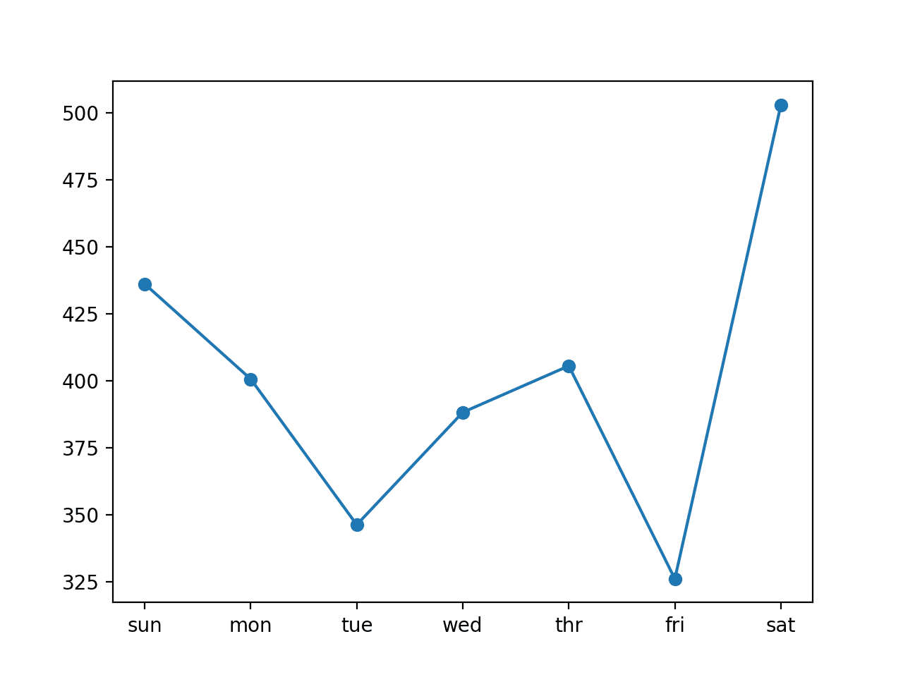
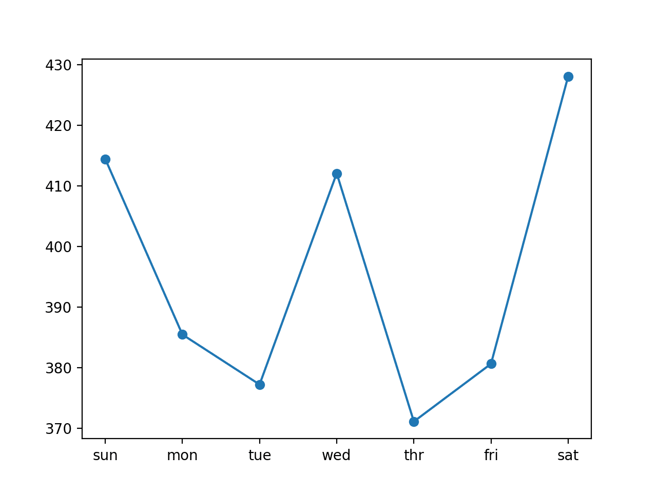
We can see that in this case, the model was skillful as compared to a naive forecast, achieving an overall RMSE of about 404 kilowatts, less than 465 kilowatts achieved by a naive model.
A plot of the daily RMSE is also created. The plot shows that perhaps Tuesdays and Fridays are easier days to forecast than the other days and that perhaps Saturday at the end of the standard week is the hardest day to forecast.
Line Plot of RMSE per Day for Univariate CNN with 7-day Inputs
We can increase the number of prior days to use as input from seven to 14 by changing the n_input variable.
1
2
# evaluate model and get scores
n_input=14
Re-running the example with this change first prints a summary of the performance of the model.
Note: Your results may vary given the stochastic nature of the algorithm or evaluation procedure, or differences in numerical precision. Consider running the example a few times and compare the average outcome.
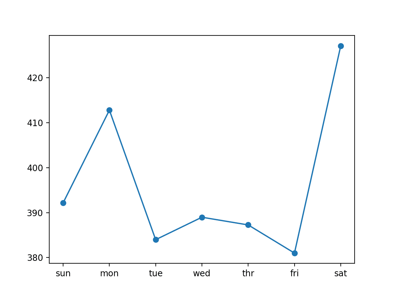
In this case, we can see a further drop in the overall RMSE, suggesting that further tuning of the input size and perhaps the kernel size of the model may result in better performance.
Comparing the per-day RMSE scores, we see some are better and some are worse than using seventh inputs.
This may suggest a benefit in using the two different sized inputs in some way, such as an ensemble of the two approaches or perhaps a single model (e.g. a multi-headed model) that reads the training data in different ways.
Line Plot of RMSE per Day for Univariate CNN with 14-day Inputs
Multi-step Time Series Forecasting With a Multichannel CNN
In this section, we will update the CNN developed in the previous section to use each of the eight time series variables to predict the next standard week of daily total power consumption.
We will do this by providing each one-dimensional time series to the model as a separate channel of input.
The CNN will then use a separate kernel and read each input sequence onto a separate set of filter maps, essentially learning features from each input time series variable.
This is helpful for those problems where the output sequence is some function of the observations at prior time steps from multiple different features, not just (or including) the feature being forecasted. It is unclear whether this is the case in the power consumption problem, but we can explore it nonetheless.
First, we must update the preparation of the training data to include all of the eight features, not just the one total daily power consumed. It requires a single line:
1
X.append(data[in_start:in_end,:])
The complete to_supervised() function with this change is listed below.
# step over the entire history one time step at a time
for_inrange(len(data)):
# define the end of the input sequence
in_end=in_start+n_input
out_end=in_end+n_out
# ensure we have enough data for this instance
ifout_end<=len(data):
X.append(data[in_start:in_end,:])
y.append(data[in_end:out_end,0])
# move along one time step
in_start+=1
returnarray(X),array(y)
We also must update the function used to make forecasts with the fit model to use all eight features from the prior time steps. Again, another small change:
We will use 14 days of prior observations across eight of the input variables as we did in the final section of the prior section that resulted in slightly better performance.
1
n_input=14
Finally, the model used in the previous section does not perform well on this new framing of the problem.
The increase in the amount of data requires a larger and more sophisticated model that is trained for longer.
With a little trial and error, one model that performs well uses two convolutional layers with 32 filter maps followed by pooling, then another convolutional layer with 16 feature maps and pooling. The fully connected layer that interprets the features is increased to 100 nodes and the model is fit for 70 epochs with a batch size of 16 samples.
The updated build_model() function that defines and fits the model on the training dataset is listed below.
Running the example fits and evaluates the model, printing the overall RMSE across all seven days, and the per-day RMSE for each lead time.
Note: Your results may vary given the stochastic nature of the algorithm or evaluation procedure, or differences in numerical precision. Consider running the example a few times and compare the average outcome.
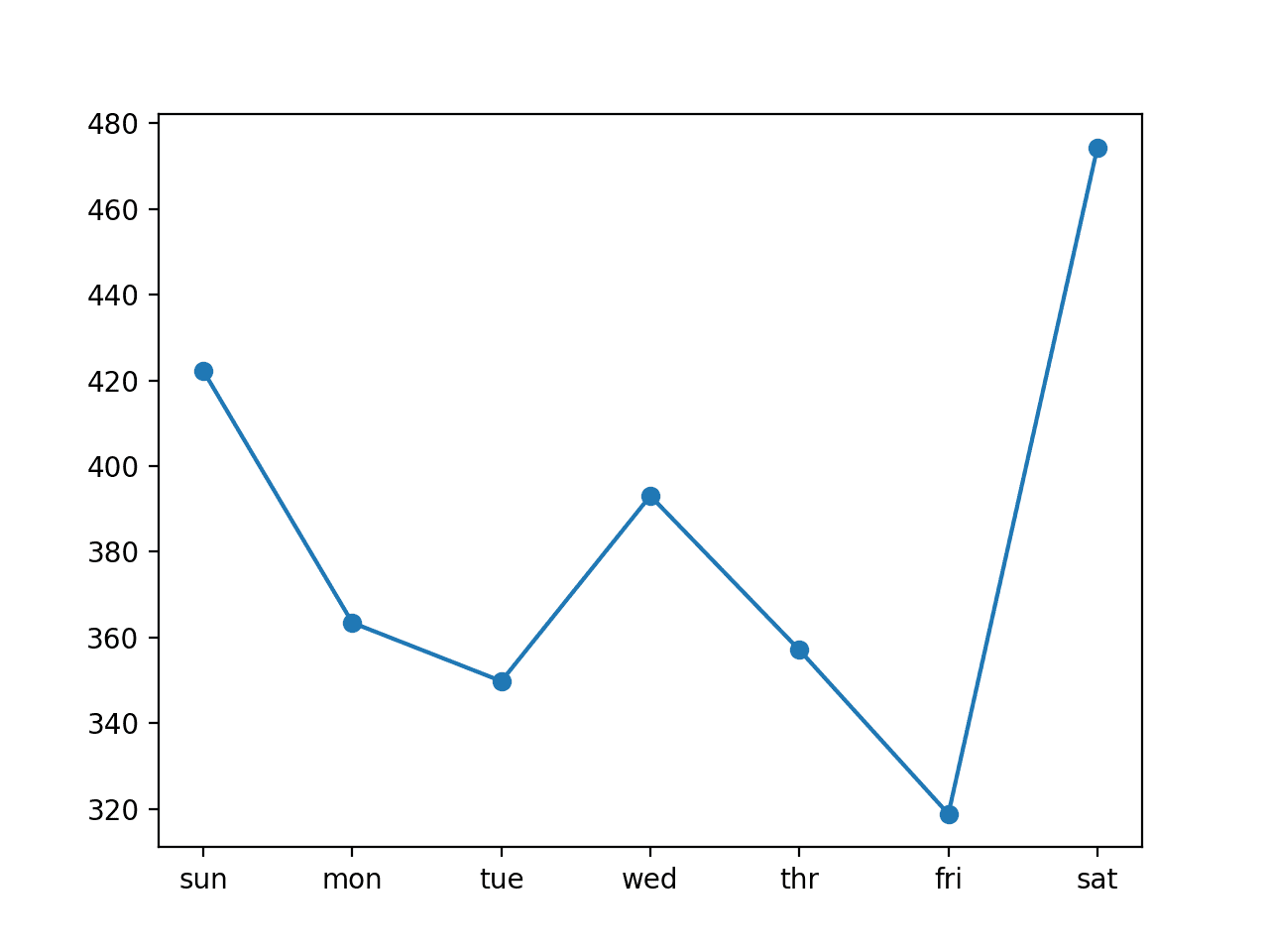
We can see that in this case, the use of all eight input variables does result in another small drop in the overall RMSE score.
For the daily RMSE scores, we do see that some are better and some are worse than the univariate CNN from the previous section.
The final day, Saturday, remains a challenging day to forecast, and Friday an easy day to forecast. There may be some benefit in designing models to focus specifically on reducing the error of the harder to forecast days.
It may be interesting to see if the variance across daily scores could be further reduced with a tuned model or perhaps an ensemble of multiple different models. It may also be interesting to compare the performance for a model that uses seven or even 21 days of input data to see if further gains can be made.
Line Plot of RMSE per Day for a Multichannel CNN with 14-day Inputs
Multi-step Time Series Forecasting With a Multihead CNN
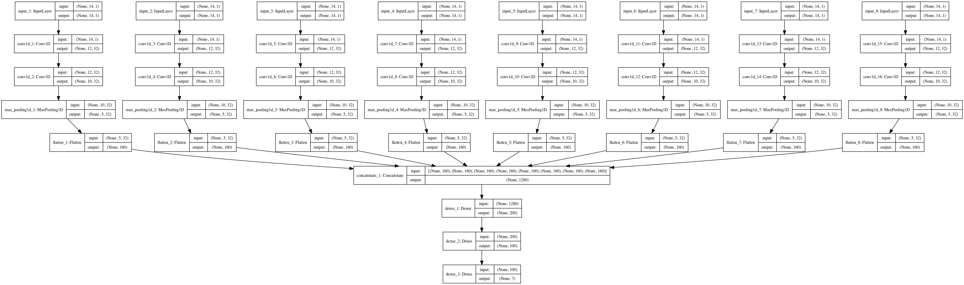
We can further extend the CNN model to have a separate sub-CNN model or head for each input variable, which we can refer to as a multi-headed CNN model.
This requires a modification to the preparation of the model, and in turn, modification to the preparation of the training and test datasets.
Starting with the model, we must define a separate CNN model for each of the eight input variables.
The configuration of the model, including the number of layers and their hyperparameters, were also modified to better suit the new approach. The new configuration is not optimal and was found with a little trial and error.
We can loop over each variable and create a sub-model that takes a one-dimensional sequence of 14 days of data and outputs a flat vector containing a summary of the learned features from the sequence. Each of these vectors can be merged via concatenation to make one very long vector that is then interpreted by some fully connected layers before a prediction is made.
As we build up the submodels, we keep track of the input layers and flatten layers in lists. This is so that we can specify the inputs in the definition of the model object and use the list of flatten layers in the merge layer.
Running the example fits and evaluates the model, printing the overall RMSE across all seven days, and the per-day RMSE for each lead time.
Note: Your results may vary given the stochastic nature of the algorithm or evaluation procedure, or differences in numerical precision. Consider running the example a few times and compare the average outcome.
We can see that in this case, the overall RMSE is skillful compared to a naive forecast, but with the chosen configuration may not perform better than the multi-channel model in the previous section.
We can also see a different, more pronounced profile for the daily RMSE scores where perhaps Mon-Tue and Thu-Fri are easier for the model to predict than the other forecast days.
These results may be useful when combined with another forecast model.
It may be interesting to explore alternate methods in the architecture for merging the output of each sub-model.
Line Plot of RMSE per Day for a Multi-head CNN with 14-day Inputs
Extensions
This section lists some ideas for extending the tutorial that you may wish to explore.
Size of Input. Explore more or fewer numbers of days used as input for the model, such as three days, 21 days, 30 days and more.
Model Tuning. Tune the structure and hyperparameters for a model and further lift model performance on average.
Data Scaling. Explore whether data scaling, such as standardization and normalization, can be used to improve the performance of any of the CNN models.
Learning Diagnostics. Use diagnostics such as learning curves for the train and validation loss and mean squared error to help tune the structure and hyperparameters of a CNN model.
Vary Kernel Size. Combine the multichannel CNN with the multi-headed CNN and use a different kernel size for each head to see if this configuration can further improve performance.
If you explore any of these extensions, I’d love to know.
Further Reading
This section provides more resources on the topic if you are looking to go deeper.
Hi Jason, thanks for the tutorial. One naive question: for last complete code, how to make prediction fixed / reproducible ? I tried “from numpy.random import seed” “seed(1)”, but the scores are still varied when running twice.
Great article – thank you for the code examples. I really enjoy looking at your work since I’m trying to learn ML/DL. Question – what if I wanted to forecast out all of the variables separately rather than one total daily power consumption?
This would be a multi-step multi-variate problem. I show how in my book.
I would recommend treating it like a seq2seq problem and forecast n variables for each step in the output sequence. An encoder-decoder model would be appropriate with a CNN or LSTM input model.
Hi. When you increase the number of training example by overlapping your data, do you not run the risk of overfitting your model? You are essentially giving the model the same data multiple times.
For the multi channel model (using 8 inputs, with 2 convo layers pooling , 1 convo and pooling), you actually get an error when using n_input = 7. Do you have any idea?
The error is actually
Negative dimension size caused by subtracting 3 from 1 for ‘conv1d_55/convolution/Conv2D’ (op: ‘Conv2D’) with input shapes: [?,1,1,32], [1,3,32,16].
Hi, kim and Josom. When using the model and n_input = 7 , I encountered the same problem, how do you solve it?
“Negative dimension size caused by subtracting 3 from 1 for ‘conv1d_55/convolution/Conv2D’ (op: ‘Conv2D’) with input shapes: [?,1,1,32], [1,3,32,16].”
Thanks Jason, i believe that the feature map is too small for the layers, which resulted in the error.
Also, one point to note is that my multi channel model is not doing as well as your example. (stochastic). However, it is actually doing worst than the single variable model with n_input = 21!
Hi Jason,
First of all congratulations and many thanks for the tutorials! I have some question:
In the first example with the univariate CNN in evaluate_model function you wrote “history = [x for x in train]”. Why? Shouldn’t be something like “history = [x for x in test]” since we want to evaluate the model?
If I use the to_supervised function also for the test set and then make prediction as follows:
Hi Jason, as always great tutorial ! I had a question concerning the multi-head CNN, would it be a good idea to use different CNN architecture instead of using the same one ?
Hi Jason, thanks for these examples. Do you see a difference between the results in using multi-channel vs multi-head CNN for multi-variate data? What is your recommendation on using these 2 different approaches?
Try both, see work works for you. I like multi-head with multi-channel so that I can use different kernel sizes on the same data – much like a resnet type design.
Thank you for this tutorial and for the book version as well. I tried to plot observations against predictions for a given time step with the date in the x-axis but couldn’t get it right. Could you please help with that. Thank you!
Thank you for your reply. May be I wasn’t clear, it’s not about the plot itself but how to extract predictions for each time step to be able to plot against the observation. (e.g forecasts of just 1-day lead) against the test set which is test[:, :, 0]. thanks
Hi Jason, thank you so much for your tutorial. it helped me a lot.. I have tried this code on my data (speed data during a sequence of time) and it works very well. However, i need to run Resnet on the same data, i have replaced the def ‘build_model’ by a residual block but it did not work. Please, have you idea what should i change in your code to have residual neural network ?? if you have already an example, it will be great.. Thanks a lot for your support.
Thanks for the great tutorial! I wonder if the multivariate channel approach is applicable for high-dimensional data, e.g. for 100 variables that could effect the outcome?
I am working on it but I get confused about the “history” you are using. I don’t get why you don’t just use the test data to predict y_hat_sequence. To me it seems like you append sample i of the test set to history (line 117 in the first 2 examples) and then you predict on the last 7 days of history, which is sample i of the test set.
Please tell me where the error in reasoning is..
Hi.. I used 70/30 for train and test to predict forecast on my data using CNN. How can I predict day ahead or hour ahead prediction. Should I use walk forward validation?
I am currently trying to apply the Multi-step Time Series Forecasting With a Univariate CNN and i am facing troubles with the batch size and input shapes.
My data are very few at the moment, 30 days of 1440 timesteps each day of a sensor measurement . my goal is to predict another day , so another 1440 timesteps. The input_shape i am using is (30, 1440 , 1) so on the Conv1D layer i put on input_shape = (1440, 1).
Then basically i followed your instructions on how to structure the rest of the network to see how it works but i get an error when i run it ( with any number of batch size).
Is it something obvious that i am doing wrong?
Should i use different shapes?
Thank you in advance for your time and your extremely helpful tutorials i have used before. Apologies if it is something obsolete or something out of your knowledge.
This is the error in case that aids your understanding :
—————————————————————————
ValueError Traceback (most recent call last)
in
16 # fit network
17 #model.summary()
—> 18 model.fit(train, y_train, epochs=epochs, verbose=verbose, batch_size =2)
I’m coming from your tutorial on Multivariate, multi-step (e.g. 20 day loopback) time series forecasting using LSTM neural networks.
I’d like to compare the LSTM results to the CNN results here. Do you mind explaining how I could use the reframed data from that example to apply to apply to this example here for daily prediction?
I have a question (it might be silly). What about if you only have data corresponding to several months of each year instead of the 12 months. You dont have continuous data for that period of time or let’s just assume you dont care about all the months (perhaps season time series analysis). The data for this particular problem was collected between December 2006 and November 2010, let’s say you only want to study April through July of each year, i.e., you would have 4 months for each year (2007,2008,2009,2010). The first approach that comes to my mind is to treat each year as a different problem and just create a model for each one them (or use the same model) and compare results. I imagine there are approaches out there to “combine” that type of data and use the data of each year all together. I am assuming we cant just “stack” data, i.e., after July of 2007, we cant just have April of 2008, because probably the values from July might not be useful to predict April values.
Do you have any suggestions? (Sorry if you have addressed this issue on another post, if so please let me know which one)
Thanks for replying. I dont understand what you meant by modeling with what I have.
If I have data collected for x number of months from y different years (lets say 3 months), I am assuming I have 3 time series. Each time-series being the data collected from those x number of months corresponding to each year.
Is there a way to combine those time series into a single dataset? Or it doesnt make sense at all to combine them?
What about if you are only interested on the power consumption during summer months and you want to use the data from multiple years?
Or what about if you are only given data from certain period of the years instead of the 12 months?
Yes, if the 3 years are contiguous and observe the same feature, then it is one time series that spans 3 years.
You can frame the problem anyway you wish, and I would encourage you to get creative.
E.g. you could develop a model to only predict the interval of interest, or develop a general model and apply it to the interval of interest, etc. Test a few methods and discover what works best for your needs.
Great article on time series thanks. I was wondering how you would deal with multiple step time series in the case where the steps are not contiguous time. For example one series could be value value1, 7 days ago, value2 25 days ago, value3 33 days ago, for predicting value 4 90 days ago. Then value1 2 days ago, value2 5 days ago, value3 7 days ago for predicting value 4 20 days ago, etc. Should the time be a features read in parallel then ( a bit like a 2D image), or should there b2 2 parallel CONV1D network being pooled at later step? thanks for your opinion.
Yes, you can try modeling as-is as a first step, then try using zero padding to make the intervals uniform and a masking layer to skip the padding (for LSTM models).
I managed to apply your method to my project now, thanks for the tutorial.
but im wondering what the time it takes to train new data in production, how can I reduce the the processing time? in my case, the training time was around 30mins with GPU. any pointers will be apreciated.
1. I believe that the Y here is the The total active power consumed by the household (kilowatts), am I right? then in this snippet would be 0 ->> y.append(data[in_end:out_end, 0]). if I have Y in the last column, would it be -1 then?
2. im interested in comparing the predicted value and the actual one in a graph for a given timestep predicition. could you please tell me how to do it?
In that context, we are working with the univariate time series, as stated in the titled “Multi-step Time Series Forecasting With a Univariate CNN”. There would be only one feature.
Yes, you can use the fit model to make a prediction, e.g. model.predict() and compare the output to the expected value.
I am new to machine learning, sorry if I ask dumb question 🙂
just to clarify, I’m building a model for multivariate (15) features, Y is located in the last column (index 15th). I tried this as per your suggestion:
if out_end <= len(data):
X.append(data[in_start:in_end, :])
y.append(data[in_end:out_end, -1])
We have many rows of data, but in this tutorial we want to work with consistent weeks that start on one day and end on another (sun-sat, or mon-sun or something).
The data does not have this structure, so we clip off a row that start and some rows off the end to ensure we have this structure – so that we only have full weeks.
We also split these consistent weeks of data into a train and test set.
The number refers to a number of rows in the data.
Thank you very much for your great effort and tutorials. I have learned very much from your tutorials.
I want to predict the price of electricity and I have only time series of electric price and time series of electric load. For example, I have 1000 days of electric prices and loads. But I want to forecast the price of electricity for the next 14 days WITHOUT SUBMITTING ANY X VALUES. For example how can I forecast the price of electricity for the day-1001, day-1002, day-1003, …., day-1014 if I do not know the values of any dependent value (x_values) for the future?
In your “forecast()” function you have written such code:
yhat = pipeline.predict(x_input)[0]
But what will I do if I have not any x_input for the future days. I ask this question especially for CNN, ANN, RNN (LSTM), Direct or Recursive MultiStep Forecasting etc.
Focus on the framing of the problem, what are the inputs to the model you will have at prediction time, and what do you need from the model for one prediction.
Once this is defined, prepare your data to match then fit a model to do it.
the data i have is in seconds you have used weekly data and split accordingly train = array(split(train, len(train)/7). plz tell me how to split my data which is in seconds.
You can frame the problem any way you wish. I recommend experimenting with a few different approaches to see what works best for your specific dataset.
I have data in seconds means it changes every seconds what window size should I use???? As you restructure the data in weekly timeframe…. How to restructure my data which is in seconds… Plz help
hello,
where does this number 465 come from and how to build the “naive forecast”?
We can see that in this case, the model was skillful as compared to a naive forecast, achieving an overall RMSE of about 404 kilowatts, less than 465 kilowatts achieved by a naive model.
two more things:
1 . how to plot an actual vs predicted plot for the Multi-step Time Series Forecasting With a Multichannel CNN example?
2. where you decide which feature shall be forecasted. The last layer is model.add(Dense(N_OUTPUTS)) but N_OUTPUTS refers to the time steps that shall be predicted ahead? Or is this model outputting a forecast for each feature (column)?
You can use the plot() function from matplitlib to create a line plot of real observations, then add a plot of predictions to the same figure.
The output layer defines the number of predictions to make. For multiple variables, you can use an encoder-decoder in which the repeatvector layer defines output time steps and the output layer of the model defines the features.
thanks yes how to plot is not the issue more what.
in this concrete example: Multi-step Time Series Forecasting With a Multichannel CNN, how to retrieve the correct values. in the evaluate_forecasts function there is mse = mean_squared_error(actual[:, i], predicted[:, i]) but plotting actual or predicted returns a plot with multiple lines not quite what i expected!?
Could you please respond with a concrete example / a few lines of code, appreciate it.
PS:
shouldn’t history = [x for x in train] be history = [x for x in test] in the evaluate_model function?
i got it figured out if anyone else struggle with the same situation, the key is that the predictions array is shape (n_samples, n_timesteps, n_columns). Just plotting it will result in the picture shown above.
correct is to extract only one time step from each prediction like so: predictions[: , -1] and same for the input_X
now the result is a nice “actual vs. predicted” plot reusing the calculations made anyways in evaluate_model(), only modification, make forecast() return also x_input.
How can I determine which column of data I want to predict?I didn’t see you give the parameters to predict the global _acitve_power.I just saw it. Throw some data filter filter maxpooling flatten and looping, and so on and then output the results.
At the same time, I still have doubts about this
merged = concatenate(out_layers)
Why connect it as a one-dimensional array? Is it just for formatting to facilitate the following input? They are made up of seven different variables, so can they be combined without distinction?
Thank you for your reading. I will be waiting for your reply all the time
Has this article ever changed?I hav’t saw the graph “Structure of the Multi Headed Convolutional Neural Network” before. This graph shows that eight variables from input_1 to input_8.and then be conv1D、max_pooling、flattened.And then connect them together,We didn’t say anything about their relationship. and then Dense to (None,7),Who we are going to predict, it has not been explained,On the far right?So what are the functions of our original data? Eight variables have experienced the same changes. Why do we predict global_active_power instead of other variables, such as voltage.
I’m sorry I’m so rude,I’m just going crazy because of this.Is there any neural network articles can you recommend? I want to learn more.
Great tutorial. I have implemented a 1D cnn with similar architecture to this one, however I do first order difference and scaling between 0 and 1 and using relu.
– My model is making negative predictions. Have something like that happen to you before? I am predicting a percentage so I should not have negative values after reversing normalization and first order difference.
– You have two dense layers. The last one has the dimension of the output. How you select the number of neurons for the the previous dense layer?
How do you think I can have the net give me a range output instead o point forecasting. I was thinking of using the softmax function but wasn’t sure how that would turn out here.
Great tutorial. But i didn’t get one thing: why the result of chapter “Multi-step Time Series Forecasting With a Univariate CNN” is “Line Plot of RMSE per Day for Univariate CNN with 7-day Inputs”? How I can get the “Line Plot of ACTIVE POWER FORECAST per Day for Univariate CNN”?
Hi Jason,
Again me. Can you explain me what is the difference between filter и kernel_size in Conv1D settings. How do the filter and the kernel_size work in code?
With your settings (filter = 16 and kernel_size=3) I have got this plot: https://imgur.com/a/4MM310r (blue – prediction, orange – fact).
I want to improve my forecast model, which parameter I need to change for the better result?
Me neither. I saw it in an article, in which the author mentioned that he would test a TCN, In order to improve the results obtained with RNN. But thanks for reply !!
Hi Jason, is it possible to do a binary multistep forecast? Like a classification problem?
I am confused in how many neurons should have the last layer since in your examples the last layer have n_output neurons. In classification problem if im not wrong the last layer has the number of classes (if binary it would be 2). How would be in a binary multistep forecast?
Thanks in advance. I hope I made myself clear.
Yes, it would be the same as a numeric multi-step forecast, only the activation function would be sigmoid instead of linear and the loss function would be binary cross entropy.
I have been trying to replicate the codes in Jupyter library and so far I have encountered error on every step or line of code. Are you able to give any advice on this. I am new to python also.
Thanks to your advice, If we use Walk-Forward Validation for regression purpose, then should we scale train and validation(both features and target) for each step of prediction, because when we would like to use inverse_transform(), but the size of data for each step will be changed(for train set I mean).
OR we should not scale data in each step; I think calling whole data(fit_transform on the train and transform on test) and pass them to each step logically is wrong, is not it?
Thank you for the great tutorial. I was wondering if you could please provide some guidance on energy disaggregation using deep learning. In particular, I have the following labelled data for each 15min window of the day:
total/aggregate energy usage
appliance 1 energy usage
appliance 2 energy usage
:
appliance n energy usage
other/unknown energy usage.
Therefore, I have 96 such rows of data for each day, over 1 year for multiple homes. I would like to train a deep learning model for energy disaggregation (i.e. given the 15min aggregate energy measurements over the day, predict the DAILY appliance usage). Would you recommend a similar approach to this article for the problem. Can we use CNN or RNN for this problem.
Many thanks.
I believe you can try to build a model and see how accurate is it. Every dataset is different and hence it is hard to say it in general a model works or not. But the nature of CNN applied to time series is to look at a window while RNN is to scan across the entire time series at one time step at a time. Think whether the nature of a model makes sense to your data or problem. That would be a good way to find where to start.
Concerning my problem, my n_input =1, n_out=1, n_timesteps =1, and n_features = 20.
I use StandardScaler right after # split into standard weeks in def split_dataset(data) like train = scaler.fit_transform(train), test = scaler.transform(test)
then, I implement scaler.inverse_transform for both test and predictions in def evaluate_model(train, test, n_input) like predictions=scaler.inverse_transform(predictions), test = scaler.inverse_transform(test)
I encounter challenge like: “ValueError: non-broadcastable output operand with shape (361,1) doesn’t match the broadcast shape (361,20)”
Hello Jason! Thank you for this – it has been so much help! One thing I’m not understanding is for evaluate_forecasts(actual, predicted), where is the actual coming from? I am having shape issues with ‘actual’ within that function, because I am using a dataset that has shape (x,y) whereas the data for the tutorial has shape (x,y,z). To better understand the issue I have been trying to figure out exactly what ‘actual’ looks like, but I haven’t been able to figure out where it’s coming from.
Any insight is greatly appreciated! 🙂
For more context I am using a dataset that has monthly data, and I am not splitting it into larger chunks like this tutorial does by turning daily data into weekly chunks.
i am a beginner and I am running the same code of multistep time series forecasting in google colab with same data as you gave. but it is continuouly showing the error “TypeError Traceback (most recent call last)
/usr/local/lib/python3.10/dist-packages/numpy/lib/shape_base.py in split(ary, indices_or_sections, axis)
866 try:
–> 867 len(indices_or_sections)
868 except TypeError:
TypeError: object of type ‘float’ has no len()
During handling of the above exception, another exception occurred:” and I am unable to solve it and where the fault is Please help me.


Hi Jason, thanks for the tutorial. One naive question: for last complete code, how to make prediction fixed / reproducible ? I tried “from numpy.random import seed” “seed(1)”, but the scores are still varied when running twice.
This is a common question that I answer here:
https://machinelearningmastery.com/faq/single-faq/what-value-should-i-set-for-the-random-number-seed
Great article – thank you for the code examples. I really enjoy looking at your work since I’m trying to learn ML/DL. Question – what if I wanted to forecast out all of the variables separately rather than one total daily power consumption?
Thank you in advance.
This would be a multi-step multi-variate problem. I show how in my book.
I would recommend treating it like a seq2seq problem and forecast n variables for each step in the output sequence. An encoder-decoder model would be appropriate with a CNN or LSTM input model.
Thank you for the response Jason. Which one of your books are you referring to?
This book:
https://machinelearningmastery.com/deep-learning-for-time-series-forecasting/
Hi. When you increase the number of training example by overlapping your data, do you not run the risk of overfitting your model? You are essentially giving the model the same data multiple times.
It may, this is why we are so reliant on the model validation method.
Please teach us capsnet.
Thanks for the suggestion.
Why do you want to use capsule networks? They seem fringe to me.
Thank you – I have purchased your ebook.
Thanks for your support Jim.
For the multi channel model (using 8 inputs, with 2 convo layers pooling , 1 convo and pooling), you actually get an error when using n_input = 7. Do you have any idea?
The error is actually
Negative dimension size caused by subtracting 3 from 1 for ‘conv1d_55/convolution/Conv2D’ (op: ‘Conv2D’) with input shapes: [?,1,1,32], [1,3,32,16].
Perhaps the configuration of the model requires change in concert with changes to the input?
Hi, kim and Josom. When using the model and n_input = 7 , I encountered the same problem, how do you solve it?
“Negative dimension size caused by subtracting 3 from 1 for ‘conv1d_55/convolution/Conv2D’ (op: ‘Conv2D’) with input shapes: [?,1,1,32], [1,3,32,16].”
Thanks Jason, i believe that the feature map is too small for the layers, which resulted in the error.
Also, one point to note is that my multi channel model is not doing as well as your example. (stochastic). However, it is actually doing worst than the single variable model with n_input = 21!
Interesting.
Hi Jason,
First of all congratulations and many thanks for the tutorials! I have some question:
In the first example with the univariate CNN in evaluate_model function you wrote “history = [x for x in train]”. Why? Shouldn’t be something like “history = [x for x in test]” since we want to evaluate the model?
If I use the to_supervised function also for the test set and then make prediction as follows:
test_x, test_y = array(X), array(y)
# forecast the next week
yhat = model.predict(test_x, verbose=0)
…………
………..
score, scores = evaluate_forecasts(test_y, yhat)
Would it be correct?
Thanks
Andrea
Yes, but we need input for the first prediction of the test set, which will/may come from the end of the training set.
Thanks for the reply!
hi jason! how to download “household_power_consumption.zip” ?
because when i click that, the website cannot be open.
The link works for me.
Here is a second download location:
https://raw.githubusercontent.com/jbrownlee/Datasets/master/household_power_consumption.zip
Hi Jason,
As my understanding, song classification is a case of Time Series data right? Can you write a topic about that?
Thank you
Thanks for the suggestion.
Hi Jason, as always great tutorial ! I had a question concerning the multi-head CNN, would it be a good idea to use different CNN architecture instead of using the same one ?
Thank you
Madriss
It really depends on the problem. Perhaps try it and compare results.
Hi Jason,
I noticed that loss was very high during training.Loss must approach 0 in some task.
Ideally, but this is not always possible or even desirable if the model is overfitting.
After normalizing features,loss approach 0.
If normalizing features,how to invert scaling for actual and forecast in Walk-Forward Validation.
I am very doubtful about this, especially the CNN model in this post.
Can you give me some advice?
Thanks!
If you use sklearn to normalize, it offers an inverse_transform() function to returns data to the original scale.
If you scale manually, you can write a manual function to invert the transform.
Perhaps this will help:
https://machinelearningmastery.com/machine-learning-data-transforms-for-time-series-forecasting/
Hi Jason, thanks for these examples. Do you see a difference between the results in using multi-channel vs multi-head CNN for multi-variate data? What is your recommendation on using these 2 different approaches?
Hmm, good question.
Try both, see work works for you. I like multi-head with multi-channel so that I can use different kernel sizes on the same data – much like a resnet type design.
Hi Jason, do you have any recommendations on when multi-channel and when multi-head approach would be better?
I recommend using multi-channel and compare it to multichannel on multi-heads to allow the use of different kernel sizes.
Hi Jason
Can you provide link of code how time series data can be converted to image form for input to CNN?
Anf how to convert in 2D?
Sorry, I don’t have an example of this.
There is no need, a 1D CNN can operate on the data directly and performs very well!
i run your 2 codes and it give this error
‘array split does not result in an equal division’)
ValueError: array split does not result in an equal division
Sorry to hear that, I have some suggestions here:
https://machinelearningmastery.com/faq/single-faq/why-does-the-code-in-the-tutorial-not-work-for-me
Same error encountered as Danial..Code is not working!
I can confirm all examples work.
Please confirm that you are using Python 3.6 or higher, Keras 2.3 and TensorFlow 2.
Please also confirm that you copied all of the code exactly and ran the example from the command line.
Thank you for this tutorial and for the book version as well. I tried to plot observations against predictions for a given time step with the date in the x-axis but couldn’t get it right. Could you please help with that. Thank you!
Sorry, I don’t have the capacity to review and debug your code.
I have many posts on how to plot time series, perhaps start here:
https://machinelearningmastery.com/start-here/#timeseries
Perhaps try posting your code and error to stackoverflow?
Thank you for your reply. May be I wasn’t clear, it’s not about the plot itself but how to extract predictions for each time step to be able to plot against the observation. (e.g forecasts of just 1-day lead) against the test set which is test[:, :, 0]. thanks
You can make predictions with model.predict()
I even provide a forecast function for you in the tutorial.
Perhaps I still don’t understand the problem that you are having?
Hi Jason, thank you so much for your tutorial. it helped me a lot.. I have tried this code on my data (speed data during a sequence of time) and it works very well. However, i need to run Resnet on the same data, i have replaced the def ‘build_model’ by a residual block but it did not work. Please, have you idea what should i change in your code to have residual neural network ?? if you have already an example, it will be great.. Thanks a lot for your support.
Perhaps you can use the pre-fit model:
https://keras.io/applications/#resnet50
Thanks for the great tutorial! I wonder if the multivariate channel approach is applicable for high-dimensional data, e.g. for 100 variables that could effect the outcome?
Yes, it might be effective. Try it and see?
I am working on it but I get confused about the “history” you are using. I don’t get why you don’t just use the test data to predict y_hat_sequence. To me it seems like you append sample i of the test set to history (line 117 in the first 2 examples) and then you predict on the last 7 days of history, which is sample i of the test set.
Please tell me where the error in reasoning is..
I am using walk-forward validation, which is a preferred approach for evaluating time series forecasting models.
You can learn more here:
https://machinelearningmastery.com/backtest-machine-learning-models-time-series-forecasting/
Hi.. I used 70/30 for train and test to predict forecast on my data using CNN. How can I predict day ahead or hour ahead prediction. Should I use walk forward validation?
Walk forward validation is really only for evaluating a model.
You fit the model on all available data and make a prediction via model.predict().
Hello Jason,
I am currently trying to apply the Multi-step Time Series Forecasting With a Univariate CNN and i am facing troubles with the batch size and input shapes.
My data are very few at the moment, 30 days of 1440 timesteps each day of a sensor measurement . my goal is to predict another day , so another 1440 timesteps. The input_shape i am using is (30, 1440 , 1) so on the Conv1D layer i put on input_shape = (1440, 1).
Then basically i followed your instructions on how to structure the rest of the network to see how it works but i get an error when i run it ( with any number of batch size).
Is it something obvious that i am doing wrong?
Should i use different shapes?
Thank you in advance for your time and your extremely helpful tutorials i have used before. Apologies if it is something obsolete or something out of your knowledge.
This is the error in case that aids your understanding :
—————————————————————————
ValueError Traceback (most recent call last)
in
16 # fit network
17 #model.summary()
—> 18 model.fit(train, y_train, epochs=epochs, verbose=verbose, batch_size =2)
c:\users\hark\anaconda3\envs\tf\lib\site-packages\keras\engine\training.py in fit(self, x, y, batch_size, epochs, verbose, callbacks, validation_split, validation_data, shuffle, class_weight, sample_weight, initial_epoch, steps_per_epoch, validation_steps, **kwargs)
950 sample_weight=sample_weight,
951 class_weight=class_weight,
–> 952 batch_size=batch_size)
953 # Prepare validation data.
954 do_validation = False
c:\users\hark\anaconda3\envs\tf\lib\site-packages\keras\engine\training.py in _standardize_user_data(self, x, y, sample_weight, class_weight, check_array_lengths, batch_size)
787 feed_output_shapes,
788 check_batch_axis=False, # Don’t enforce the batch size.
–> 789 exception_prefix=’target’)
790
791 # Generate sample-wise weight values given the
sample_weightandc:\users\hark\anaconda3\envs\tf\lib\site-packages\keras\engine\training_utils.py in standardize_input_data(data, names, shapes, check_batch_axis, exception_prefix)
126 ‘: expected ‘ + names[i] + ‘ to have ‘ +
127 str(len(shape)) + ‘ dimensions, but got array ‘
–> 128 ‘with shape ‘ + str(data_shape))
129 if not check_batch_axis:
130 data_shape = data_shape[1:]
ValueError: Error when checking target: expected dense_45 to have 2 dimensions, but got array with shape (1440, 30, 1)
The error suggests a mismatch between the shape of your data and the expected shape of the model.
You can reshape the data or change the expectation of the model.
Hi Jason,
I’m coming from your tutorial on Multivariate, multi-step (e.g. 20 day loopback) time series forecasting using LSTM neural networks.
I’d like to compare the LSTM results to the CNN results here. Do you mind explaining how I could use the reframed data from that example to apply to apply to this example here for daily prediction?
You can use data with the same structure for evaluating RNNs and CNNs directly.
Hi Jason,
First of all thanks for your posts and books!
I have a question (it might be silly). What about if you only have data corresponding to several months of each year instead of the 12 months. You dont have continuous data for that period of time or let’s just assume you dont care about all the months (perhaps season time series analysis). The data for this particular problem was collected between December 2006 and November 2010, let’s say you only want to study April through July of each year, i.e., you would have 4 months for each year (2007,2008,2009,2010). The first approach that comes to my mind is to treat each year as a different problem and just create a model for each one them (or use the same model) and compare results. I imagine there are approaches out there to “combine” that type of data and use the data of each year all together. I am assuming we cant just “stack” data, i.e., after July of 2007, we cant just have April of 2008, because probably the values from July might not be useful to predict April values.
Do you have any suggestions? (Sorry if you have addressed this issue on another post, if so please let me know which one)
Thanks 🙂
Model with what you have and compare results to a naive method to see if you can develop a model that has skill.
Thanks for replying. I dont understand what you meant by modeling with what I have.
If I have data collected for x number of months from y different years (lets say 3 months), I am assuming I have 3 time series. Each time-series being the data collected from those x number of months corresponding to each year.
Is there a way to combine those time series into a single dataset? Or it doesnt make sense at all to combine them?
What about if you are only interested on the power consumption during summer months and you want to use the data from multiple years?
Or what about if you are only given data from certain period of the years instead of the 12 months?
Yes, if the 3 years are contiguous and observe the same feature, then it is one time series that spans 3 years.
You can frame the problem anyway you wish, and I would encourage you to get creative.
E.g. you could develop a model to only predict the interval of interest, or develop a general model and apply it to the interval of interest, etc. Test a few methods and discover what works best for your needs.
Hi Jason,
Great article on time series thanks. I was wondering how you would deal with multiple step time series in the case where the steps are not contiguous time. For example one series could be value value1, 7 days ago, value2 25 days ago, value3 33 days ago, for predicting value 4 90 days ago. Then value1 2 days ago, value2 5 days ago, value3 7 days ago for predicting value 4 20 days ago, etc. Should the time be a features read in parallel then ( a bit like a 2D image), or should there b2 2 parallel CONV1D network being pooled at later step? thanks for your opinion.
Yes, you can try modeling as-is as a first step, then try using zero padding to make the intervals uniform and a masking layer to skip the padding (for LSTM models).
Interesting, thanks Jason.
Hi Jason,
I managed to apply your method to my project now, thanks for the tutorial.
but im wondering what the time it takes to train new data in production, how can I reduce the the processing time? in my case, the training time was around 30mins with GPU. any pointers will be apreciated.
You can train on less data, use a smaller model, or use a faster machine.
Hi Jason,
I have two questions:
1. I believe that the Y here is the The total active power consumed by the household (kilowatts), am I right? then in this snippet would be 0 ->> y.append(data[in_end:out_end, 0]). if I have Y in the last column, would it be -1 then?
2. im interested in comparing the predicted value and the actual one in a graph for a given timestep predicition. could you please tell me how to do it?
In that context, we are working with the univariate time series, as stated in the titled “Multi-step Time Series Forecasting With a Univariate CNN”. There would be only one feature.
Yes, you can use the fit model to make a prediction, e.g. model.predict() and compare the output to the expected value.
for the graph actual vs predicted result, is this covered in your ebook time series multivariate multistep?
No, but it may be covered in some of these more introductory tutorials:
https://machinelearningmastery.com/start-here/#timeseries
For example this one:
https://machinelearningmastery.com/time-series-data-visualization-with-python/
I am new to machine learning, sorry if I ask dumb question 🙂
just to clarify, I’m building a model for multivariate (15) features, Y is located in the last column (index 15th). I tried this as per your suggestion:
if out_end <= len(data):
X.append(data[in_start:in_end, :])
y.append(data[in_end:out_end, -1])
am i doing right?
Time series with RNNs and CNNs is more complex than other models. I recommend reading this first:
https://machinelearningmastery.com/faq/single-faq/what-is-the-difference-between-samples-timesteps-and-features-for-lstm-input
HI Jason:
I have a quick questions why do you use in the split data, data[1:-328] for train and [-328:-6] for test?
To break the data into 7-day weeks.
Hi
sorry to keep asking, but I don’t understand where the number 1 -328 comes from neither does the -328and -6
Thank you
Laura
No problem Laura.
We have many rows of data, but in this tutorial we want to work with consistent weeks that start on one day and end on another (sun-sat, or mon-sun or something).
The data does not have this structure, so we clip off a row that start and some rows off the end to ensure we have this structure – so that we only have full weeks.
We also split these consistent weeks of data into a train and test set.
The number refers to a number of rows in the data.
If using array indexes and slices/ranges is new to you, see this post:
https://machinelearningmastery.com/index-slice-reshape-numpy-arrays-machine-learning-python/
Hi, Jason.
Thank you very much for your great effort and tutorials. I have learned very much from your tutorials.
I want to predict the price of electricity and I have only time series of electric price and time series of electric load. For example, I have 1000 days of electric prices and loads. But I want to forecast the price of electricity for the next 14 days WITHOUT SUBMITTING ANY X VALUES. For example how can I forecast the price of electricity for the day-1001, day-1002, day-1003, …., day-1014 if I do not know the values of any dependent value (x_values) for the future?
In your “forecast()” function you have written such code:
yhat = pipeline.predict(x_input)[0]
But what will I do if I have not any x_input for the future days. I ask this question especially for CNN, ANN, RNN (LSTM), Direct or Recursive MultiStep Forecasting etc.
Thanks for your help.
most of your tutoral
Focus on the framing of the problem, what are the inputs to the model you will have at prediction time, and what do you need from the model for one prediction.
Once this is defined, prepare your data to match then fit a model to do it.
the data i have is in seconds you have used weekly data and split accordingly train = array(split(train, len(train)/7). plz tell me how to split my data which is in seconds.
You can frame the problem any way you wish. I recommend experimenting with a few different approaches to see what works best for your specific dataset.
I have data in seconds means it changes every seconds what window size should I use???? As you restructure the data in weekly timeframe…. How to restructure my data which is in seconds… Plz help
hello,
where does this number 465 come from and how to build the “naive forecast”?
We can see that in this case, the model was skillful as compared to a naive forecast, achieving an overall RMSE of about 404 kilowatts, less than 465 kilowatts achieved by a naive model.
See this tutorial:
https://machinelearningmastery.com/naive-methods-for-forecasting-household-electricity-consumption/
Awesome got it!
two more things:
1 . how to plot an actual vs predicted plot for the Multi-step Time Series Forecasting With a Multichannel CNN example?
2. where you decide which feature shall be forecasted. The last layer is model.add(Dense(N_OUTPUTS)) but N_OUTPUTS refers to the time steps that shall be predicted ahead? Or is this model outputting a forecast for each feature (column)?
You can use the plot() function from matplitlib to create a line plot of real observations, then add a plot of predictions to the same figure.
The output layer defines the number of predictions to make. For multiple variables, you can use an encoder-decoder in which the repeatvector layer defines output time steps and the output layer of the model defines the features.
thanks yes how to plot is not the issue more what.
in this concrete example: Multi-step Time Series Forecasting With a Multichannel CNN, how to retrieve the correct values. in the evaluate_forecasts function there is mse = mean_squared_error(actual[:, i], predicted[:, i]) but plotting actual or predicted returns a plot with multiple lines not quite what i expected!?
Could you please respond with a concrete example / a few lines of code, appreciate it.
PS:
shouldn’t history = [x for x in train] be history = [x for x in test] in the evaluate_model function?
Yes, call model.predict() to get predictions, there are tens of examples on the blog for example:
https://machinelearningmastery.com/start-here/#deep_learning_time_series
We must seed history with train, then step through test one time step at a time.
thanks for the answer i think there is a misunderstanding, What is not clear to me yet is:
When i do the following:
train_x, train_y = to_supervised(train, n_input)
and than:
plt.plot(train_y [-10:])
than the result looks like this:
https://i.imgur.com/RyCmMJq.png
expected would be a single line, same for the predictions array!?
Perhaps check the shape of the data you are trying to plot?
I think you’re expecting a univariate series, and getting a multivariate series?
i got it figured out if anyone else struggle with the same situation, the key is that the predictions array is shape (n_samples, n_timesteps, n_columns). Just plotting it will result in the picture shown above.
correct is to extract only one time step from each prediction like so: predictions[: , -1] and same for the input_X
now the result is a nice “actual vs. predicted” plot reusing the calculations made anyways in evaluate_model(), only modification, make forecast() return also x_input.
Well done, happy to hear that!
How can I determine which column of data I want to predict?I didn’t see you give the parameters to predict the global _acitve_power.I just saw it. Throw some data filter filter maxpooling flatten and looping, and so on and then output the results.
At the same time, I still have doubts about this
merged = concatenate(out_layers)
Why connect it as a one-dimensional array? Is it just for formatting to facilitate the following input? They are made up of seven different variables, so can they be combined without distinction?
Thank you for your reading. I will be waiting for your reply all the time
In general, perhaps use this framework:
https://machinelearningmastery.com/how-to-define-your-machine-learning-problem/
In practice, it is typically the far right column.
Each variable operates like a separate “channel” to the 1d CNN. Does that help?
Has this article ever changed?I hav’t saw the graph “Structure of the Multi Headed Convolutional Neural Network” before. This graph shows that eight variables from input_1 to input_8.and then be conv1D、max_pooling、flattened.And then connect them together,We didn’t say anything about their relationship. and then Dense to (None,7),Who we are going to predict, it has not been explained,On the far right?So what are the functions of our original data? Eight variables have experienced the same changes. Why do we predict global_active_power instead of other variables, such as voltage.
I’m sorry I’m so rude,I’m just going crazy because of this.Is there any neural network articles can you recommend? I want to learn more.
It has always been there.
It is a complex model and probably does not make sense for many datasets.
This might help understand multi-input models:
https://machinelearningmastery.com/keras-functional-api-deep-learning/
I have read the framework you recommended to me, but I still don’t know much about this network
This might also help, it is where I got the idea:
https://machinelearningmastery.com/develop-n-gram-multichannel-convolutional-neural-network-sentiment-analysis/
HI Jason,
Great tutorial. I have implemented a 1D cnn with similar architecture to this one, however I do first order difference and scaling between 0 and 1 and using relu.
– My model is making negative predictions. Have something like that happen to you before? I am predicting a percentage so I should not have negative values after reversing normalization and first order difference.
– You have two dense layers. The last one has the dimension of the output. How you select the number of neurons for the the previous dense layer?
Thanks in advance,
Yes, it is predicting “differenced values” by your design. Use linear activation in the output nodes.
The number of nodes in the output layer matches the number of predictions to make for one sample.
Hi Jason,
Do you have an example to show how to use multistep timeseries using seq2seq in CNN?
The above tutorial gives an example of multi-step forecasting with a 1D CNN.
Hi Jason,
How do you think I can have the net give me a range output instead o point forecasting. I was thinking of using the softmax function but wasn’t sure how that would turn out here.
Thank you
You could use an ensemble of regression models to get a distribution of point predictions, called a prediction interval.
HI Jason,
Great tutorial. But i didn’t get one thing: why the result of chapter “Multi-step Time Series Forecasting With a Univariate CNN” is “Line Plot of RMSE per Day for Univariate CNN with 7-day Inputs”? How I can get the “Line Plot of ACTIVE POWER FORECAST per Day for Univariate CNN”?
You can make a single prediction with model.predict(). Then given the predicted array call the plot() function from matplot lib to plot the forecast.
If plotting a time series is new for you, see this introductory tutorial:
https://machinelearningmastery.com/load-explore-time-series-data-python/
Hi Jason,
Again me. Can you explain me what is the difference between filter и kernel_size in Conv1D settings. How do the filter and the kernel_size work in code?
With your settings (filter = 16 and kernel_size=3) I have got this plot: https://imgur.com/a/4MM310r (blue – prediction, orange – fact).
I want to improve my forecast model, which parameter I need to change for the better result?
There is no formula for improving performance, instead you must use systematic experimentation to discover what works best.
The suggestions here will help:
https://machinelearningmastery.com/start-here/#better
As for what kernels mean, see this:
https://machinelearningmastery.com/convolutional-layers-for-deep-learning-neural-networks/
Hi Json,
After we getting the Mean RMSE and individuals as,
cnn: [1300.269] 1308.5, 1300.8, 1305.1, 1296.6, 1307.7, 1290.3, 1292.7
n_input = 1000
split_rate = 0.70
kernel_size = 50
epochs = 450
batch_size = 100
How can we calculate the Model Accuracy?
Is there any specific equation?
Thank you
We cannot calculate accuracy for regression:
https://machinelearningmastery.com/faq/single-faq/how-do-i-calculate-accuracy-for-regression
Hi Json,
Thank you for the reply.
I saw that R-Squared can measure the regression accuracy (but for linear models). But this is a non-linear model.
Is there any method to say about the model accuracy. Are RMSE values enough for saying how a model is predicting the things accurately?
Please help.
Thank you.
You must choose a metric that best captures what is important about a model for you or your project stakeholders.
Okay Json, Thank you
You’re welcome.
Dear Jason,
Thanks for this excellent book.
I have juts finished it, it took me about 3,5 weeks, and I have written a review of the book here:
http://questioneurope.blogspot.com/2020/07/deep-learning-for-time-series.html
Kind regards,
Dominique
Thanks Dominique, well done on your progress!
Hi Jason,
Is this approach the same as the Temporal Convolutional Networks(TCN) also used for sequence modeling tasks?
I’m not familiar with TCN, sorry. What is it exactly?
Me neither. I saw it in an article, in which the author mentioned that he would test a TCN, In order to improve the results obtained with RNN. But thanks for reply !!
def split_dataset(data):
# split into standard weeks
train, test = data[1:-328], data[-328:-6]
why train begin from [1:-328 not [0:-328].
why you skipped the first entry?
To work with the data in complete “weeks” of data.
Perhaps re-read the section that describes how we split up the data.
Hi Jason, is it possible to do a binary multistep forecast? Like a classification problem?
I am confused in how many neurons should have the last layer since in your examples the last layer have n_output neurons. In classification problem if im not wrong the last layer has the number of classes (if binary it would be 2). How would be in a binary multistep forecast?
Thanks in advance. I hope I made myself clear.
Thanks. Have a great day.
Yes, it would be the same as a numeric multi-step forecast, only the activation function would be sigmoid instead of linear and the loss function would be binary cross entropy.
This is gold man. Thanks for sharing. Gonna try some stuffs over here.
Love your blog!
Thanks!
Hi Jason,
Thank you for providing this example.
I have been trying to replicate the codes in Jupyter library and so far I have encountered error on every step or line of code. Are you able to give any advice on this. I am new to python also.
You’re welcome.
I recommend not using a notebook – they cause problems for nearly everyone:
https://machinelearningmastery.com/faq/single-faq/why-dont-use-or-recommend-notebooks
Hi Jason,
Thanks to your advice, If we use Walk-Forward Validation for regression purpose, then should we scale train and validation(both features and target) for each step of prediction, because when we would like to use inverse_transform(), but the size of data for each step will be changed(for train set I mean).
OR we should not scale data in each step; I think calling whole data(fit_transform on the train and transform on test) and pass them to each step logically is wrong, is not it?
I really appreciate any help you can provide.
You’re welcome.
Scaling the inputs and target are generally a good idea for regression and time series forecasting.
Hello Jason. Thank you for this tutorial, it is very much appreciated.
I wonder; if I want to expand on your tutorial and do a prediction for 30 days instead, what do I need to change/consider? And why?
Perhaps you can reframe the dataset to have 30 output values in a sample, then adjust the model to make this prediction.
Or, perhaps you can use a model that predicts a few time steps in a recursive manner.
Perhaps try a few approaches and discover what works best for your specific dataset.
Hello Jason,
Thank you for the great tutorial. I was wondering if you could please provide some guidance on energy disaggregation using deep learning. In particular, I have the following labelled data for each 15min window of the day:
total/aggregate energy usage
appliance 1 energy usage
appliance 2 energy usage
:
appliance n energy usage
other/unknown energy usage.
Therefore, I have 96 such rows of data for each day, over 1 year for multiple homes. I would like to train a deep learning model for energy disaggregation (i.e. given the 15min aggregate energy measurements over the day, predict the DAILY appliance usage). Would you recommend a similar approach to this article for the problem. Can we use CNN or RNN for this problem.
Many thanks.
I believe you can try to build a model and see how accurate is it. Every dataset is different and hence it is hard to say it in general a model works or not. But the nature of CNN applied to time series is to look at a window while RNN is to scan across the entire time series at one time step at a time. Think whether the nature of a model makes sense to your data or problem. That would be a good way to find where to start.
Hi Jason,
Concerning my problem, my n_input =1, n_out=1, n_timesteps =1, and n_features = 20.
I use StandardScaler right after # split into standard weeks in def split_dataset(data) like train = scaler.fit_transform(train), test = scaler.transform(test)
then, I implement scaler.inverse_transform for both test and predictions in def evaluate_model(train, test, n_input) like predictions=scaler.inverse_transform(predictions), test = scaler.inverse_transform(test)
I encounter challenge like: “ValueError: non-broadcastable output operand with shape (361,1) doesn’t match the broadcast shape (361,20)”
Any suggestion of how to handle the error above.
Many thanks!
Hello Jason! Thank you for this – it has been so much help! One thing I’m not understanding is for evaluate_forecasts(actual, predicted), where is the actual coming from? I am having shape issues with ‘actual’ within that function, because I am using a dataset that has shape (x,y) whereas the data for the tutorial has shape (x,y,z). To better understand the issue I have been trying to figure out exactly what ‘actual’ looks like, but I haven’t been able to figure out where it’s coming from.
Any insight is greatly appreciated! 🙂
Hi Sarah…the following resource may help with reshaping issues. This tutorial discusses LSTMs, however it is also applicable for CNNs.
https://machinelearningmastery.com/reshape-input-data-long-short-term-memory-networks-keras/
For more context I am using a dataset that has monthly data, and I am not splitting it into larger chunks like this tutorial does by turning daily data into weekly chunks.
Hello Jashon,
Its great to see your article.
i am a beginner and I am running the same code of multistep time series forecasting in google colab with same data as you gave. but it is continuouly showing the error “TypeError Traceback (most recent call last)
/usr/local/lib/python3.10/dist-packages/numpy/lib/shape_base.py in split(ary, indices_or_sections, axis)
866 try:
–> 867 len(indices_or_sections)
868 except TypeError:
TypeError: object of type ‘float’ has no len()
During handling of the above exception, another exception occurred:” and I am unable to solve it and where the fault is Please help me.
Hi Vineet…You are very welcome! Would it be possible to install Anaconda on your local machine and try the implementation?
https://machinelearningmastery.com/setup-python-environment-machine-learning-deep-learning-anaconda/