Batch normalization is a technique designed to automatically standardize the inputs to a layer in a deep learning neural network.
Once implemented, batch normalization has the effect of dramatically accelerating the training process of a neural network, and in some cases improves the performance of the model via a modest regularization effect.
In this tutorial, you will discover how to use batch normalization to accelerate the training of deep learning neural networks in Python with Keras.
After completing this tutorial, you will know:
How to create and configure a BatchNormalization layer using the Keras API.
How to add the BatchNormalization layer to deep learning neural network models.
How to update an MLP model to use batch normalization to accelerate training on a binary classification problem.
Kick-start your project with my new book Better Deep Learning, including step-by-step tutorials and the Python source code files for all examples.
Let’s get started.
Updated Oct/2019: Updated for Keras 2.3 and TensorFlow 2.0.
How to Accelerate Learning of Deep Neural Networks With Batch Normalization Photo by Angela and Andrew, some rights reserved.
Tutorial Overview
This tutorial is divided into three parts; they are:
BatchNormalization in Keras
BatchNormalization in Models
BatchNormalization Case Study
BatchNormalization in Keras
Keras provides support for batch normalization via the BatchNormalization layer.
For example:
1
bn=BatchNormalization()
The layer will transform inputs so that they are standardized, meaning that they will have a mean of zero and a standard deviation of one.
During training, the layer will keep track of statistics for each input variable and use them to standardize the data.
Further, the standardized output can be scaled using the learned parameters of Beta and Gamma that define the new mean and standard deviation for the output of the transform. The layer can be configured to control whether these additional parameters will be used or not via the “center” and “scale” attributes respectively. By default, they are enabled.
The statistics used to perform the standardization, e.g. the mean and standard deviation of each variable, are updated for each mini batch and a running average is maintained.
A “momentum” argument allows you to control how much of the statistics from the previous mini batch to include when the update is calculated. By default, this is kept high with a value of 0.99. This can be set to 0.0 to only use statistics from the current mini-batch, as described in the original paper.
1
bn=BatchNormalization(momentum=0.0)
At the end of training, the mean and standard deviation statistics in the layer at that time will be used to standardize inputs when the model is used to make a prediction.
The default configuration estimating mean and standard deviation across all mini batches is probably sensible.
Want Better Results with Deep Learning?
Take my free 7-day email crash course now (with sample code).
Click to sign-up and also get a free PDF Ebook version of the course.
BatchNormalization in Models
Batch normalization can be used at most points in a model and with most types of deep learning neural networks.
Input and Hidden Layer Inputs
The BatchNormalization layer can be added to your model to standardize raw input variables or the outputs of a hidden layer.
Batch normalization is not recommended as an alternative to proper data preparation for your model.
Nevertheless, when used to standardize the raw input variables, the layer must specify the input_shape argument; for example:
1
2
3
4
...
model=Sequential
model.add(BatchNormalization(input_shape=(2,)))
...
When used to standardize the outputs of a hidden layer, the layer can be added to the model just like any other layer.
1
2
3
4
5
...
model=Sequential
...
model.add(BatchNormalization())
...
Use Before or After the Activation Function
The BatchNormalization normalization layer can be used to standardize inputs before or after the activation function of the previous layer.
The original paper that introduced the method suggests adding batch normalization before the activation function of the previous layer, for example:
1
2
3
4
5
6
...
model=Sequential
model.add(Dense(32))
model.add(BatchNormalization())
model.add(Activation('relu'))
...
Some reported experiments suggest better performance when adding the batch normalization layer after the activation function of the previous layer; for example:
1
2
3
4
5
...
model=Sequential
model.add(Dense(32,activation='relu'))
model.add(BatchNormalization())
...
If time and resources permit, it may be worth testing both approaches on your model and use the approach that results in the best performance.
Let’s take a look at how batch normalization can be used with some common network types.
MLP Batch Normalization
The example below adds batch normalization after the activation function between Dense hidden layers.
1
2
3
4
5
6
7
8
# example of batch normalization for an mlp
from keras.layers import Dense
from keras.layers import BatchNormalization
...
model.add(Dense(32,activation='relu'))
model.add(BatchNormalization())
model.add(Dense(1))
...
CNN Batch Normalization
The example below adds batch normalization after the activation function between a convolutional and max pooling layers.
1
2
3
4
5
6
7
8
9
10
11
12
# example of batch normalization for an cnn
from keras.layers import Dense
from keras.layers import Conv2D
from keras.layers import MaxPooling2D
from keras.layers import BatchNormalization
...
model.add(Conv2D(32,(3,3),activation='relu'))
model.add(Conv2D(32,(3,3),activation='relu'))
model.add(BatchNormalization())
model.add(MaxPooling2D())
model.add(Dense(1))
...
RNN Batch Normalization
The example below adds batch normalization after the activation function between an LSTM and Dense hidden layers.
1
2
3
4
5
6
7
8
9
# example of batch normalization for a lstm
from keras.layers import Dense
from keras.layers import LSTM
from keras.layers import BatchNormalization
...
model.add(LSTM(32))
model.add(BatchNormalization())
model.add(Dense(1))
...
BatchNormalization Case Study
In this section, we will demonstrate how to use batch normalization to accelerate the training of an MLP on a simple binary classification problem.
This example provides a template for applying batch normalization to your own neural network for classification and regression problems.
Binary Classification Problem
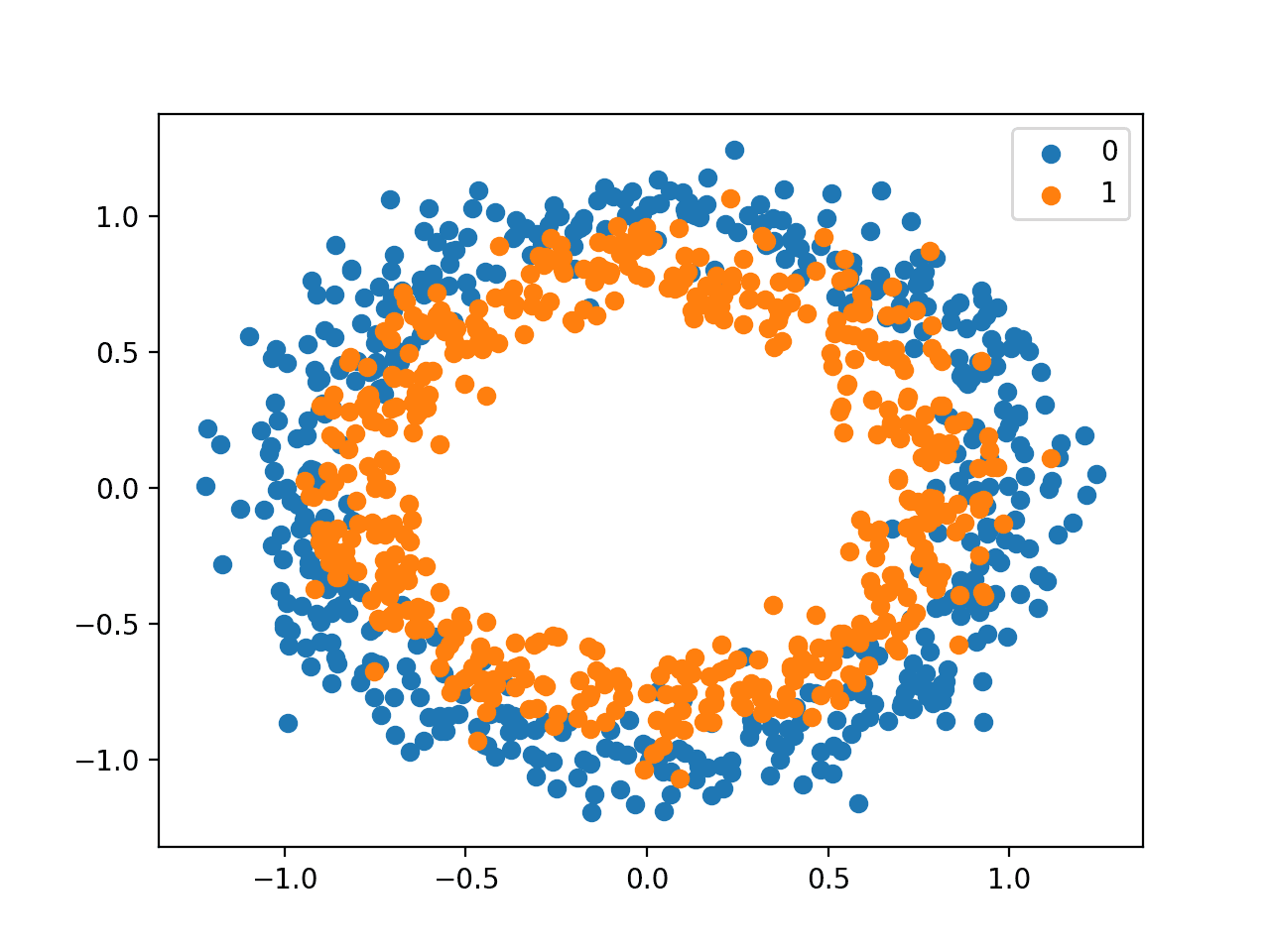
We will use a standard binary classification problem that defines two two-dimensional concentric circles of observations, one circle for each class.
Each observation has two input variables with the same scale and a class output value of either 0 or 1. This dataset is called the “circles” dataset because of the shape of the observations in each class when plotted.
We can use the make_circles() function to generate observations from this problem. We will add noise to the data and seed the random number generator so that the same samples are generated each time the code is run.
We can plot the dataset where the two variables are taken as x and y coordinates on a graph and the class value is taken as the color of the observation.
The complete example of generating the dataset and plotting it is listed below.
1
2
3
4
5
6
7
8
9
10
11
12
# scatter plot of the circles dataset with points colored by class
Running the example creates a scatter plot showing the concentric circles shape of the observations in each class.
We can see the noise in the dispersal of the points making the circles less obvious.
Scatter Plot of Circles Dataset With Color Showing the Class Value of Each Sample
This is a good test problem because the classes cannot be separated by a line, e.g. are not linearly separable, requiring a nonlinear method such as a neural network to address.
Multilayer Perceptron Model
We can develop a Multilayer Perceptron model, or MLP, as a baseline for this problem.
First, we will split the 1,000 generated samples into a train and test dataset, with 500 examples in each. This will provide a sufficiently large sample for the model to learn from and an equally sized (fair) evaluation of its performance.
1
2
3
4
# split into train and test
n_train=500
trainX,testX=X[:n_train,:],X[n_train:,:]
trainy,testy=y[:n_train],y[n_train:]
We will define a simple MLP model. The network must have two inputs in the visible layer for the two variables in the dataset.
The model will have a single hidden layer with 50 nodes, chosen arbitrarily, and use the rectified linear activation function (ReLU) and the He random weight initialization method. The output layer will be a single node with the sigmoid activation function, capable of predicting a 0 for the outer circle and a 1 for the inner circle of the problem.
The model will be trained using stochastic gradient descent with a modest learning rate of 0.01 and a large momentum of 0.9, and the optimization will be directed using the binary cross entropy loss function.
Once defined, the model can be fit on the training dataset.
We will use the holdout test dataset as a validation dataset and evaluate its performance at the end of each training epoch. The model will be fit for 100 epochs, chosen after a little trial and error.
Running the example fits the model and evaluates it on the train and test sets.
Note: Your results may vary given the stochastic nature of the algorithm or evaluation procedure, or differences in numerical precision. Consider running the example a few times and compare the average outcome.
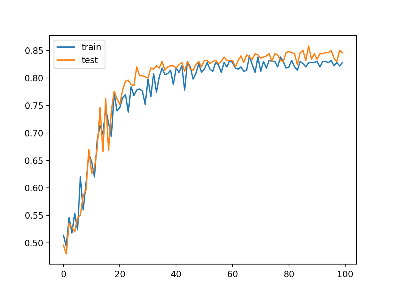
In this case, we can see that the model achieved an accuracy of about 84% on the holdout dataset and achieved comparable performance on both the train and test sets, given the same size and similar composition of both datasets.
1
Train: 0.838, Test: 0.846
A graph is created showing line plots of the classification accuracy on the train (blue) and test (orange) datasets.
The plot shows comparable performance of the model on both datasets during the training process. We can see that performance leaps up over the first 30-to-40 epochs to above 80% accuracy then is slowly refined.
Line Plot of MLP Classification Accuracy on Train and Test Datasets Over Training Epochs
This result, and specifically the dynamics of the model during training, provide a baseline that can be compared to the same model with the addition of batch normalization.
MLP With Batch Normalization
The model introduced in the previous section can be updated to add batch normalization.
The expectation is that the addition of batch normalization would accelerate the training process, offering similar or better classification accuracy of the model in fewer training epochs. Batch normalization is also reported as providing a modest form of regularization, meaning that it may also offer a small reduction in generalization error demonstrated by a small increase in classification accuracy on the holdout test dataset.
A new BatchNormalization layer can be added to the model after the hidden layer before the output layer. Specifically, after the activation function of the prior hidden layer.
Running the example first prints the classification accuracy of the model on the train and test dataset.
Note: Your results may vary given the stochastic nature of the algorithm or evaluation procedure, or differences in numerical precision. Consider running the example a few times and compare the average outcome.
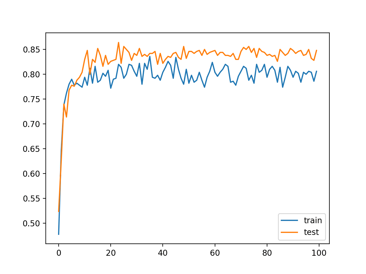
In this case, we can see comparable performance of the model on both the train and test set of about 84% accuracy, very similar to what we saw in the previous section, if not a little bit better.
1
Train: 0.846, Test: 0.848
A graph of the learning curves is also created showing classification accuracy on both the train and test sets for each training epoch.
In this case, we can see that the model has learned the problem faster than the model in the previous section without batch normalization. Specifically, we can see that classification accuracy on the train and test datasets leaps above 80% within the first 20 epochs, as opposed to 30-to-40 epochs in the model without batch normalization.
The plot also shows the effect of batch normalization during training. We can see lower performance on the training dataset than the test dataset: scores on the training dataset that are lower than the performance of the model at the end of the training run. This is likely the effect of the input collected and updated each mini-batch.
Line Plot Classification Accuracy of MLP With Batch Normalization After Activation Function on Train and Test Datasets Over Training Epochs
We can also try a variation of the model where batch normalization is applied prior to the activation function of the hidden layer, instead of after the activation function.
Running the example first prints the classification accuracy of the model on the train and test dataset.
Note: Your results may vary given the stochastic nature of the algorithm or evaluation procedure, or differences in numerical precision. Consider running the example a few times and compare the average outcome.
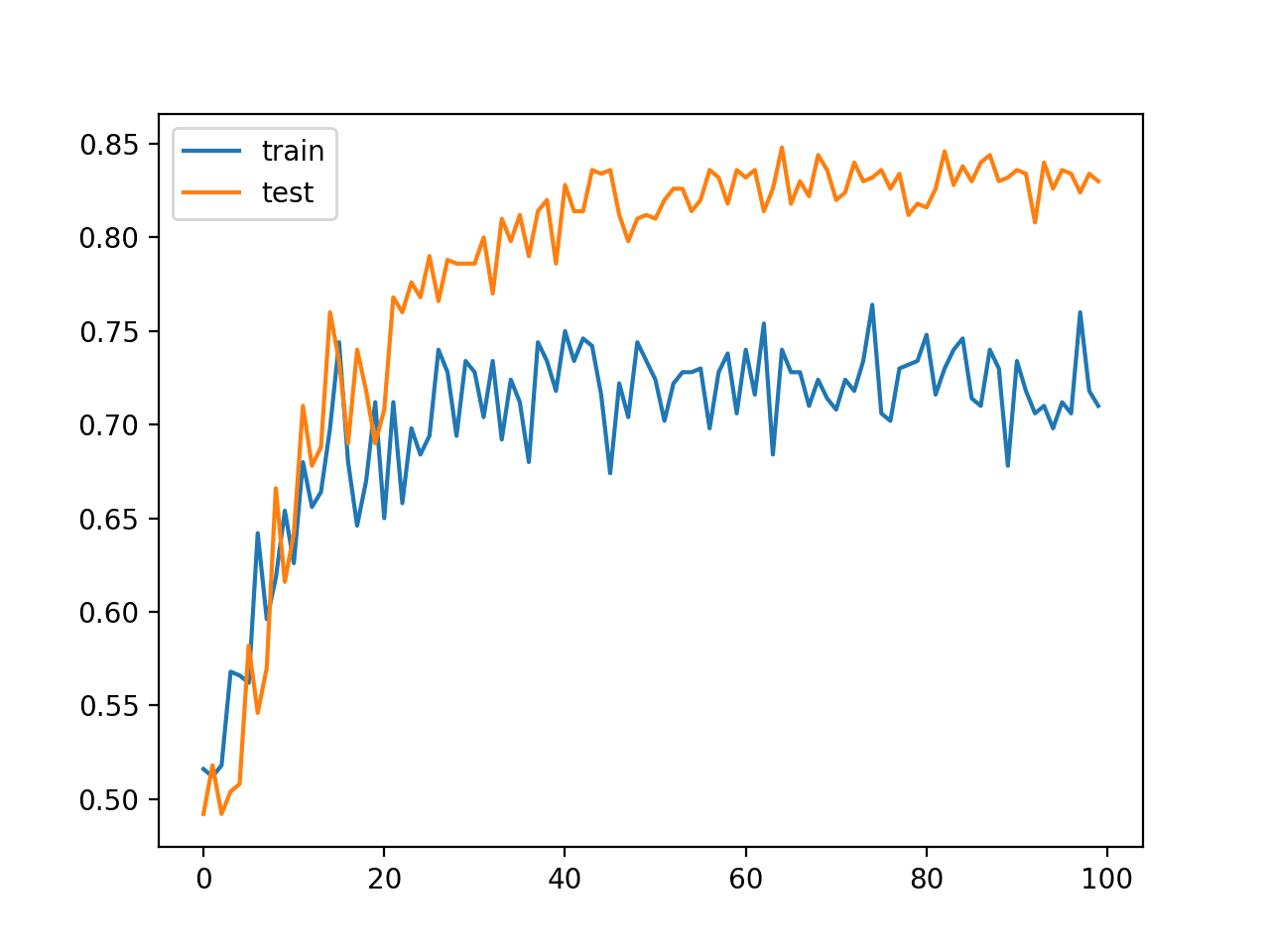
In this case, we can see comparable performance of the model on the train and test datasets, but slightly worse than the model without batch normalization.
1
Train: 0.826, Test: 0.830
The line plot of the learning curves on the train and test sets also tells a different story.
The plot shows the model learning perhaps at the same pace as the model without batch normalization, but the performance of the model on the training dataset is much worse, hovering around 70% to 75% accuracy, again likely an effect of the statistics collected and used over each mini-batch.
At least for this model configuration on this specific dataset, it appears that batch normalization is more effective after the rectified linear activation function.
Line Plot Classification Accuracy of MLP With Batch Normalization Before Activation Function on Train and Test Datasets Over Training Epochs
Extensions
This section lists some ideas for extending the tutorial that you may wish to explore.
Without Beta and Gamma. Update the example to not use the beta and gamma parameters in the batch normalization layer and compare results.
Without Momentum. Update the example to not use momentum in the batch normalization layer during training and compare results.
Input Layer. Update the example to use batch normalization after the input to the model and compare results.
If you explore any of these extensions, I’d love to know.
Further Reading
This section provides more resources on the topic if you are looking to go deeper.
I thought batch normalization is to scale values near [-1,1], so I thought there’s no need to add BN if the lstm output is already [-1, 1]? Could you please say more about the benefits to apply BN after tanh or sigmoid?
Hello!, I understand that it is to keep stable the first two empirical moments of the distribution of the activations, so that the neuron/node does not spend effort in learning that distribution. The original paper says that
Something that is not clear is whether one can use batch normalization instead of preprocessing. I mean, normally before feeding the data in the network, you would want to standardize it first. There are various solutions for this, such as the MinMax scaler. Can we replace such methods with a simple batch normalization as the input layer in our network?
Thanks Jason. Could you be more specific why it is not recommanded to use BatchNormalization on inputs vs StandardScaler for example? I may miss a point but I don’t see the difference.
Thank you for your amazing articles and books they really help my start in machine learning .
I really need your help in a problem i’m having I wrote this code to classify documents into 20 topics using lstm it executed well and the training accuracy was 99 but the test accuracy was 7 so after research this problem it seemed it might be an over fitting problem so I tried all solutions I could found but no use (I tried dropout layers , validation split , change the optimizer change learning rate tried BN ) so this my code and I hope you can help me fix it :
docs=[]
test_d=[]
for filename in glob.glob(os.path.join(“train”, ‘*.txt’)):
with open(filename,’r’) as f:
content=f.read()
#text=map(str.rstrip, f.readlines())
#for line in content:
#line = line.replace(“\n”, “”)
content = content.split(‘\n’)
content = ” “.join(content)
docs.append(content)
embeddings_index = dict()
f = open(‘glove.6B.100d.txt’)
for line in f:
values = line.split()
word = values[0]
coefs = asarray(values[1:],)
embeddings_index[word] = coefs
f.close()
print(‘Loaded %s word vectors.’ % len(embeddings_index))
embedding_matrix = zeros((vocab_size, embedding_dim))
for word, i in t.word_index.items():
embedding_vector = embeddings_index.get(word)
if embedding_vector is not None:
embedding_matrix[i] = embedding_vector
labels=array([])
encoder = LabelEncoder()
encoder.fit(labels)
encoded_Y = encoder.transform(labels)
dummy_y = np_utils.to_categorical(encoded_Y)
model = Sequential()
e = Embedding(vocab_size, embedding_dim , weights=[embedding_matrix], input_length=max_length, trainable=False)
model.add(e)
model.add(BatchNormalization())
model.add(SpatialDropout1D(0.2))
model.add(LSTM(128, dropout=0.2, recurrent_dropout=0.2,return_sequences=True))
#model.add(LSTM(50, return_sequences=True))
model.add(Flatten())
#model.add(Dense(25, activation=’relu’))
model.add(BatchNormalization())
model.add(Dense(20, activation=’softmax’))
# compile the model
opt = adam(lr=0.8)
model.compile(optimizer=’RMSprop’, loss=’categorical_crossentropy’, metrics=[‘acc’])
# summarize the model
print(model.summary())
#class_weight = class_weight.compute_class_weight(‘balanced’,numpy.unique(dummy_y),dummy_y)
#class_weights = class_weight.compute_class_weight(‘balanced’,np.unique(np.ravel(dummy_y,order=’C’)),np.ravel(dummy_y,order=’C’))
# fit the model
model.fit(padded_docs, dummy_y, validation_split=0.30, epochs=10, verbose=2)
# evaluate the model
loss, accuracy = model.evaluate(padded_docs, dummy_y, verbose=2)
print(‘Train Accuracy: %f’ % (accuracy*100))
labels=[]
for filename in glob.glob(os.path.join(“test”, ‘*.txt’)):
with open(filename,’r’) as f:
content=f.read()
content = content.split(‘\n’)
content = ” “.join(content)
test_d.append(content)
t = Tokenizer()
t.fit_on_texts(test_d)
encoded_docs = t.texts_to_sequences(test_d)
test_d=[]
padded_docs = pad_sequences(encoded_docs, maxlen=max_length, padding=’post’)
encoder = LabelEncoder()
encoder.fit(test_labels)
encoded_Y = encoder.transform(test_labels)
# convert integers to dummy variables (i.e. one hot encoded)
dummy_y = np_utils.to_categorical(encoded_Y)
loss, accuracy = model.evaluate(padded_docs, dummy_y, verbose=2)
print(‘Test Accuracy: %f’ % (accuracy*100))
print(‘\007’)
and Thanks in advanced I would really appreciate your help .
Yes, the value will be weighted average of the prior value and the current value, e. 0.9 of this value 0.1 of the last value, giving the value some history.
A “momentum” argument allows you to control how much of the statistics from the previous mini batch to include when the update is calculated. By default, this is kept high with a value of 0.99. This can be set to 0.0 to only use statistics from the current mini-batch, as described in the original paper.
What if we use BN after pooling? what I have observed, it does not affect performance. Also would you please clarify that can we use dropout and MN simultaneously in CNN? If yes, what should be the order of implementation?
(1) Model details for implementation of CNN based Time Series Classification.
(2 )LSTM or CNN for Time Series Classification?
(3) Sequential model or Functional API model is preferred?
(4) How to augment input time series data and implement it in the proposed model?
Hi Mr Jason,
kindly explain the possible reasons for fluctuation or ziz-zag behavior in accuracy curves as visible in your all plots. In almost all materials, graph is shown smooth. However, in practical we get fluctuations. Please also give suggestions to overcome it.
or joining outputs of various convolutions in an inception module.
In general is there a resource (book / site) that focuses on custom NN architectures?
I just want to check Batch Normalisation output, given an input
For instance, given input as a numpy array: [[[1.,2,3]],[[3,4,1]]], I expect BatchNormalisation would convert it to [[[-2,0,0],[0,0,-2]]]
import numpy as np
import tensorflow as tf
from tensorflow import keras
from keras.layers import BatchNormalization
Hi jason,
your articles are great.
whenever I add batch-normalize with different momentum , the results get worse and the model fails to converge !!!!
and I have found this question repeated without an accepted solution
(the implementation with python 3.9 – sypder )


Hi Jason,
Awesome article. Well presented.
Is there any mathematical proof when to use BN before or after activation fn?
Thanks!
I have seen no proofs, the findings are empirical only – like much of applied machine learning.
Thanks!
Hi, Jason!
Why is BN applied after lstm? As the lstm output is [-1, 1] after tanh?
Thanks!
Why not?
I thought batch normalization is to scale values near [-1,1], so I thought there’s no need to add BN if the lstm output is already [-1, 1]? Could you please say more about the benefits to apply BN after tanh or sigmoid?
Thanks a lot!
I don’t recall material on the topic, perhaps refer to the original paper?
Thanks for reply ^ ^
Hello!, I understand that it is to keep stable the first two empirical moments of the distribution of the activations, so that the neuron/node does not spend effort in learning that distribution. The original paper says that
Excellent tutorial as always!
Something that is not clear is whether one can use batch normalization instead of preprocessing. I mean, normally before feeding the data in the network, you would want to standardize it first. There are various solutions for this, such as the MinMax scaler. Can we replace such methods with a simple batch normalization as the input layer in our network?
No. I recommend that you continue to prepare data correctly before modeling.
Thnak you!
So do we have do standardization( apply some scaler minmax or standard scaler) and then apply batch normalization in the sequence model?
I recommend separately considering the scaling of your input data from batch normalization.
Thanks Jason. Could you be more specific why it is not recommanded to use BatchNormalization on inputs vs StandardScaler for example? I may miss a point but I don’t see the difference.
Yes, StandardScaler gives more control over the data preparation as a separate step. Batch norm is estimating mu and sigma from each batch of samples.
Thank you for your amazing articles and books they really help my start in machine learning .
I really need your help in a problem i’m having I wrote this code to classify documents into 20 topics using lstm it executed well and the training accuracy was 99 but the test accuracy was 7 so after research this problem it seemed it might be an over fitting problem so I tried all solutions I could found but no use (I tried dropout layers , validation split , change the optimizer change learning rate tried BN ) so this my code and I hope you can help me fix it :
docs=[]
test_d=[]
for filename in glob.glob(os.path.join(“train”, ‘*.txt’)):
with open(filename,’r’) as f:
content=f.read()
#text=map(str.rstrip, f.readlines())
#for line in content:
#line = line.replace(“\n”, “”)
content = content.split(‘\n’)
content = ” “.join(content)
docs.append(content)
embeddings_index = dict()
f = open(‘glove.6B.100d.txt’)
for line in f:
values = line.split()
word = values[0]
coefs = asarray(values[1:],)
embeddings_index[word] = coefs
f.close()
print(‘Loaded %s word vectors.’ % len(embeddings_index))
embedding_matrix = zeros((vocab_size, embedding_dim))
for word, i in t.word_index.items():
embedding_vector = embeddings_index.get(word)
if embedding_vector is not None:
embedding_matrix[i] = embedding_vector
labels=array([])
encoder = LabelEncoder()
encoder.fit(labels)
encoded_Y = encoder.transform(labels)
dummy_y = np_utils.to_categorical(encoded_Y)
model = Sequential()
e = Embedding(vocab_size, embedding_dim , weights=[embedding_matrix], input_length=max_length, trainable=False)
model.add(e)
model.add(BatchNormalization())
model.add(SpatialDropout1D(0.2))
model.add(LSTM(128, dropout=0.2, recurrent_dropout=0.2,return_sequences=True))
#model.add(LSTM(50, return_sequences=True))
model.add(Flatten())
#model.add(Dense(25, activation=’relu’))
model.add(BatchNormalization())
model.add(Dense(20, activation=’softmax’))
# compile the model
opt = adam(lr=0.8)
model.compile(optimizer=’RMSprop’, loss=’categorical_crossentropy’, metrics=[‘acc’])
# summarize the model
print(model.summary())
#class_weight = class_weight.compute_class_weight(‘balanced’,numpy.unique(dummy_y),dummy_y)
#class_weights = class_weight.compute_class_weight(‘balanced’,np.unique(np.ravel(dummy_y,order=’C’)),np.ravel(dummy_y,order=’C’))
# fit the model
model.fit(padded_docs, dummy_y, validation_split=0.30, epochs=10, verbose=2)
# evaluate the model
loss, accuracy = model.evaluate(padded_docs, dummy_y, verbose=2)
print(‘Train Accuracy: %f’ % (accuracy*100))
labels=[]
for filename in glob.glob(os.path.join(“test”, ‘*.txt’)):
with open(filename,’r’) as f:
content=f.read()
content = content.split(‘\n’)
content = ” “.join(content)
test_d.append(content)
t = Tokenizer()
t.fit_on_texts(test_d)
encoded_docs = t.texts_to_sequences(test_d)
test_d=[]
padded_docs = pad_sequences(encoded_docs, maxlen=max_length, padding=’post’)
encoder = LabelEncoder()
encoder.fit(test_labels)
encoded_Y = encoder.transform(test_labels)
# convert integers to dummy variables (i.e. one hot encoded)
dummy_y = np_utils.to_categorical(encoded_Y)
loss, accuracy = model.evaluate(padded_docs, dummy_y, verbose=2)
print(‘Test Accuracy: %f’ % (accuracy*100))
print(‘\007’)
and Thanks in advanced I would really appreciate your help .
I have some suggestions here that might help:
https://machinelearningmastery.com/start-here/#better
“”A “momentum” argument allows you to control how much of the statistics from the previous mini-batch to include when the update is calculated””
Can you explain this line more clearly
Yes, the value will be weighted average of the prior value and the current value, e. 0.9 of this value 0.1 of the last value, giving the value some history.
A “momentum” argument allows you to control how much of the statistics from the previous mini batch to include when the update is calculated. By default, this is kept high with a value of 0.99. This can be set to 0.0 to only use statistics from the current mini-batch, as described in the original paper.
Paper reference?
Any book on neural nets will describe this. Perhaps start here:
https://amzn.to/36HsYfq
Hi Jason,
Have you read any best practices on where to apply Batch Normalization in a CNN? The original BN layer seems to say that BN can be applied to any layer in the CNN: https://arxiv.org/pdf/1502.03167.pdf. But there are some caveats to how BN should be applied after a convolution layer that I’m still trying to wrap my head around: https://stackoverflow.com/questions/38553927/batch-normalization-in-convolutional-neural-network. A keras example of that would be really helpful.
Yes, before pooling.
See the above example of batch norm for CNNs.
What if we use BN after pooling? what I have observed, it does not affect performance. Also would you please clarify that can we use dropout and MN simultaneously in CNN? If yes, what should be the order of implementation?
Good questions, I answer them here:
https://machinelearningmastery.com/batch-normalization-for-training-of-deep-neural-networks/
thanks for your kind support.
You’re welcome.
Further, it is requested to kindly share
(1) Model details for implementation of CNN based Time Series Classification.
(2 )LSTM or CNN for Time Series Classification?
(3) Sequential model or Functional API model is preferred?
(4) How to augment input time series data and implement it in the proposed model?
You can see most of these examples here:
https://machinelearningmastery.com/start-here/#deep_learning_time_series
Hi Mr Jason,
kindly explain the possible reasons for fluctuation or ziz-zag behavior in accuracy curves as visible in your all plots. In almost all materials, graph is shown smooth. However, in practical we get fluctuations. Please also give suggestions to overcome it.
Thanks and regards
You can fit multiple final models and ensemble their predictions to smooth out accuracy of predictions:
https://machinelearningmastery.com/how-to-reduce-model-variance/
Is there another application of BN that article does not describe when joining complex (potentially multi-input) streams in functional api?
or joining outputs of various convolutions in an inception module.
In general is there a resource (book / site) that focuses on custom NN architectures?
This can help you with learning how to code complex architectures:
https://machinelearningmastery.com/how-to-implement-major-architecture-innovations-for-convolutional-neural-networks/
Perhaps this example of the functional API can be adapted for your needs:
https://machinelearningmastery.com/keras-functional-api-deep-learning/
Hi Jason
I just want to check Batch Normalisation output, given an input
For instance, given input as a numpy array: [[[1.,2,3]],[[3,4,1]]], I expect BatchNormalisation would convert it to [[[-2,0,0],[0,0,-2]]]
import numpy as np
import tensorflow as tf
from tensorflow import keras
from keras.layers import BatchNormalization
x=np.array([[[1.,2,3]],[[3,4,1]]])
y=BatchNormalization()(x)
However, this output y is same as x
Can you please help with the code to get the normalised x using BatchNormalisation?
Recall that batch norm is standardizing input over the batch where internal coefficient are learned during training and applied during inference.
I would not expect that using the layer in the way you describe to be effective. E.g. inference directly.
Yeah, It wont be
I am studying neural networks and want to assess the output of each layer.
You can use the functional API to define a model where each layer is passed on to the next layer, and also can be used as an output layer.
This will help you get started with the functional API:
https://machinelearningmastery.com/keras-functional-api-deep-learning/
Hi jason,
your articles are great.
whenever I add batch-normalize with different momentum , the results get worse and the model fails to converge !!!!
and I have found this question repeated without an accepted solution
(the implementation with python 3.9 – sypder )
Hi Ahmed…Thank you for the feedback! The following background may help clarify:
https://machinelearningmastery.com/batch-normalization-for-training-of-deep-neural-networks/
https://towardsdatascience.com/curse-of-batch-normalization-8e6dd20bc304