Time series decomposition involves thinking of a series as a combination of level, trend, seasonality, and noise components.
Decomposition provides a useful abstract model for thinking about time series generally and for better understanding problems during time series analysis and forecasting.
In this tutorial, you will discover time series decomposition and how to automatically split a time series into its components with Python.
After completing this tutorial, you will know:
The time series decomposition method of analysis and how it can help with forecasting.
How to automatically decompose time series data in Python.
How to decompose additive and multiplicative time series problems and plot the results.
Kick-start your project with my new book Time Series Forecasting With Python, including step-by-step tutorials and the Python source code files for all examples.
Let’s get started.
Updated Apr/2019: Updated the link to dataset.
Updated Aug/2019: Updated data loading to use new API.
How to Decompose Time Series Data into Trend and Seasonality Photo by Terry Robinson, some rights reserved.
Time Series Components
A useful abstraction for selecting forecasting methods is to break a time series down into systematic and unsystematic components.
Systematic: Components of the time series that have consistency or recurrence and can be described and modeled.
Non-Systematic: Components of the time series that cannot be directly modeled.
A given time series is thought to consist of three systematic components including level, trend, seasonality, and one non-systematic component called noise.
These components are defined as follows:
Level: The average value in the series.
Trend: The increasing or decreasing value in the series.
Seasonality: The repeating short-term cycle in the series.
Noise: The random variation in the series.
Stop learning Time Series Forecasting the slow way!
Take my free 7-day email course and discover how to get started (with sample code).
Click to sign-up and also get a free PDF Ebook version of the course.
Combining Time Series Components
A series is thought to be an aggregate or combination of these four components.
All series have a level and noise. The trend and seasonality components are optional.
It is helpful to think of the components as combining either additively or multiplicatively.
Additive Model
An additive model suggests that the components are added together as follows:
1
y(t) = Level + Trend + Seasonality + Noise
An additive model is linear where changes over time are consistently made by the same amount.
A linear trend is a straight line.
A linear seasonality has the same frequency (width of cycles) and amplitude (height of cycles).
Multiplicative Model
A multiplicative model suggests that the components are multiplied together as follows:
1
y(t) = Level * Trend * Seasonality * Noise
A multiplicative model is nonlinear, such as quadratic or exponential. Changes increase or decrease over time.
A nonlinear trend is a curved line.
A non-linear seasonality has an increasing or decreasing frequency and/or amplitude over time.
Decomposition as a Tool
This is a useful abstraction.
Decomposition is primarily used for time series analysis, and as an analysis tool it can be used to inform forecasting models on your problem.
It provides a structured way of thinking about a time series forecasting problem, both generally in terms of modeling complexity and specifically in terms of how to best capture each of these components in a given model.
Each of these components are something you may need to think about and address during data preparation, model selection, and model tuning. You may address it explicitly in terms of modeling the trend and subtracting it from your data, or implicitly by providing enough history for an algorithm to model a trend if it may exist.
You may or may not be able to cleanly or perfectly break down your specific time series as an additive or multiplicative model.
Real-world problems are messy and noisy. There may be additive and multiplicative components. There may be an increasing trend followed by a decreasing trend. There may be non-repeating cycles mixed in with the repeating seasonality components.
Nevertheless, these abstract models provide a simple framework that you can use to analyze your data and explore ways to think about and forecast your problem.
The statsmodels library provides an implementation of the naive, or classical, decomposition method in a function called seasonal_decompose(). It requires that you specify whether the model is additive or multiplicative.
Both will produce a result and you must be careful to be critical when interpreting the result. A review of a plot of the time series and some summary statistics can often be a good start to get an idea of whether your time series problem looks additive or multiplicative.
The seasonal_decompose() function returns a result object. The result object contains arrays to access four pieces of data from the decomposition.
For example, the snippet below shows how to decompose a series into trend, seasonal, and residual components assuming an additive model.
The result object provides access to the trend and seasonal series as arrays. It also provides access to the residuals, which are the time series after the trend, and seasonal components are removed. Finally, the original or observed data is also stored.
1
2
3
4
5
6
7
from statsmodels.tsa.seasonal import seasonal_decompose
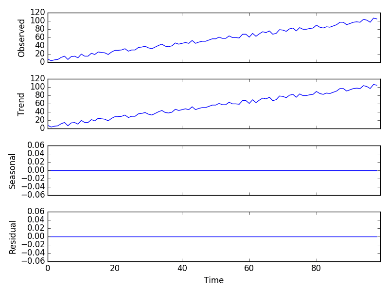
We can create a time series comprised of a linearly increasing trend from 1 to 99 and some random noise and decompose it as an additive model.
Because the time series was contrived and was provided as an array of numbers, we must specify the frequency of the observations (the period=1 argument). If a Pandas Series object is provided, this argument is not required.
1
2
3
4
5
6
7
8
from random import randrange
from pandas import Series
from matplotlib import pyplot
from statsmodels.tsa.seasonal import seasonal_decompose
Running the example creates the series, performs the decomposition, and plots the 4 resulting series.
We can see that the entire series was taken as the trend component and that there was no seasonality.
Additive Model Decomposition Plot
We can also see that the residual plot shows zero. This is a good example where the naive, or classical, decomposition was not able to separate the noise that we added from the linear trend.
The naive decomposition method is a simple one, and there are more advanced decompositions available, like Seasonal and Trend decomposition using Loess or STL decomposition.
Caution and healthy skepticism is needed when using automated decomposition methods.
Multiplicative Decomposition
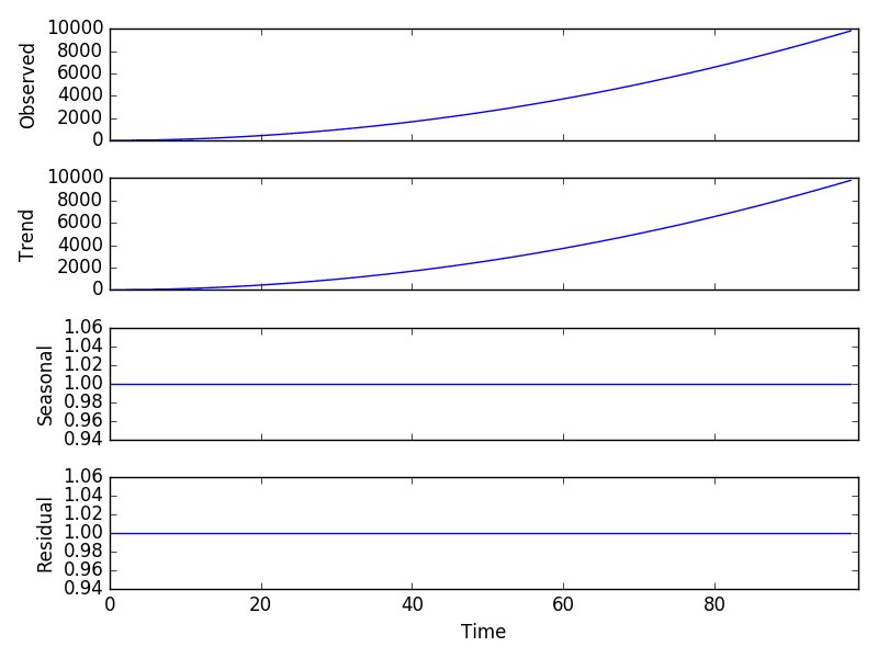
We can contrive a quadratic time series as a square of the time step from 1 to 99, and then decompose it assuming a multiplicative model.
1
2
3
4
5
6
7
from pandas import Series
from matplotlib import pyplot
from statsmodels.tsa.seasonal import seasonal_decompose
Running the example, we can see that, as in the additive case, the trend is easily extracted and wholly characterizes the time series.
Multiplicative Model Decomposition Plot
Exponential changes can be made linear by data transforms. In this case, a quadratic trend can be made linear by taking the square root. An exponential growth in seasonality may be made linear by taking the natural logarithm.
Again, it is important to treat decomposition as a potentially useful analysis tool, but to consider exploring the many different ways it could be applied for your problem, such as on data after it has been transformed or on residual model errors.
Let’s look at a real world dataset.
Airline Passengers Dataset
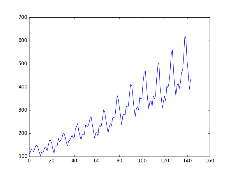
The Airline Passengers dataset describes the total number of airline passengers over a period of time.
The units are a count of the number of airline passengers in thousands. There are 144 monthly observations from 1949 to 1960.
Reviewing the line plot, it suggests that there may be a linear trend, but it is hard to be sure from eye-balling. There is also seasonality, but the amplitude (height) of the cycles appears to be increasing, suggesting that it is multiplicative.
Plot of the Airline Passengers Dataset
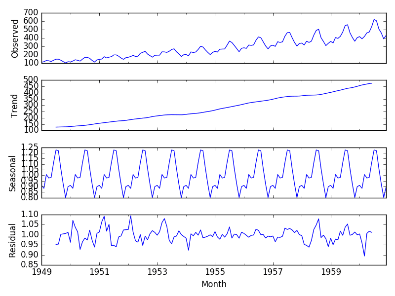
We will assume a multiplicative model.
The example below decomposes the airline passengers dataset as a multiplicative model.
1
2
3
4
5
6
7
from pandas import read_csv
from matplotlib import pyplot
from statsmodels.tsa.seasonal import seasonal_decompose
Running the example plots the observed, trend, seasonal, and residual time series.
We can see that the trend and seasonality information extracted from the series does seem reasonable. The residuals are also interesting, showing periods of high variability in the early and later years of the series.
Multiplicative Decomposition of Airline Passenger Dataset
Further Reading
This section lists some resources for further reading on time series decomposition.
In this tutorial, you discovered time series decomposition and how to decompose time series data with Python.
Specifically, you learned:
The structure of decomposing time series into level, trend, seasonality, and noise.
How to automatically decompose a time series dataset with Python.
How to decompose an additive or multiplicative model and plot the results.
Do you have any questions about time series decomposition, or about this tutorial?
Ask your questions in the comments below and I will do my best to answer.
Want to Develop Time Series Forecasts with Python?
Maybe you’ll be able to help me, I’m having some trouble with the statsmodels library. When I try to run your last example, I get this AttributeError:
“AttributeError: ‘Index’ object has no attribute ‘inferred_freq'”
I checked the dataset that was exported from DataMarket and realized that the last was this one:
“International airline passengers: monthly totals in thousands. Jan 49 ? Dec 60”
I removed it and then now a TypeError:
“TypeError: ‘numpy.float64’ object cannot be interpreted as an index”
I already tried to use this statsmodels library before, got this same error several times, gave up and started using R for that. I even asked this question o stackoverflow:
Hi Alvaro,
maybe a bit late but it hope it helps. IMHO you are getting this error as you are feeding to seasonal_decompose() a pandas Series. If so, be sure to have a datetime type in your index or it will crash. You can make a turnaoround of this behavior just by passing the Series values to a np.array() and specifying the frequency manually,
Hi Jason and Álvaro,
Thanks Jason for the detailed description step by step. Highly appreciated!
I got the same problem using notebook, Jupiter. Please let me know if you figure out the problem.
thanks!
I did the followings and although I still receive an VisibleDeprecationWarning (using a non-integer number instead of an integer will result in an error in the future return np.r_[[np.nan] * head, x, [np.nan] * tail]),
I got the plots for time series components.
– I removed the last line in the CSV file: “International airline passengers: monthly totals in thousands. Jan 49 ? Dec 60”
Thanks for copmlete explanation. Maybe stupid question but how do you explain the random % in the model. Let’s say it has random 49% in multiplicative decomposition.
A time series trace may be thought to comprise of signal and random component. We can’t model the random component, at best we can measure it and factor it into our confidence intervals.
Hello. Everything works OK when I test this dataset, but when I try to run it using data with daily temperature (from your other lesson: https://machinelearningmastery.com/time-series-seasonality-with-python/), I get the error: “ValueError: You must specify a freq or x must be a pandas object with a timeseries index witha freq not set to None”. I don’t understand why some data are not concerned as pandas object.
Yes, I understand that. The problem is that I use exactly the same piece of code for both files (data are loaded as pandas series). I want to avoid specyfing the frequency explicitly, because I would like to adapt this code to my own data, whre this freqency is unknown. Are there any specific requirements as regards CSV structure? I noticed that the file from this lesson has values for every month, whereas the other file mentioned by me has values given daily but I don’t believe it may be a reason for errors.
There are no special requirements. You may need to specify a custom function to load the date/time column, depending on whether Pandas can figure it out or not.
Using freq = 1 is what is causing the Seasonal and Residual plots to flat-line. It specifies using a moving average convolution of length 1, i.e. average over a single point.
Try setting freq = 12 (for presumed monthly data) or make the input a pandas Series and set its index to a suitably contrived DatetimeIndex.
Simple query: When I am using quarterly data-sets I loose first-2 and last-2 quarters of data in (seasonally) adjusted series. Similarly for monthly I loose first-6 and last-6 months of data?
I would like to have adjusted series which is up to current period. Is there a way to get entire adjusted data series?
Hello, your texts are very interesting and useful. But in this text, I have a question. The example with a one column of data in dataset works well, but what I need to do to use the same code column by column in a multiple column dataset? Thank you!
Is there a way to find those signals that are periodic? I have a bunch of timeseries data (timestamp, uuid). I want to find those uuids that are seasonal. Expected output must be a set of uuids and their respective timestamps.
To notch it up a bit, given a large set of datapoints, is there a way to find all seasonal data with different seasonality?
I do not know the frequency of the given data. The timestamps are in datetime format – like this – 2017-01-29 07:17:10. Their frequency could be hourly, daily, weekly…or some other frequency.
Hi, Jason, very clear and helpful article.
I noticed that in the Airline Passengers example, seasonal and reside data ,first several values and last several values are lost. Is this a flaw of the algorithm?
if it is , any suggestion to fix this? cause usually people want to detect the most recent abnormal data instead of the historical ones.
the number of obs is the same, but first and last three values are nan in that example.
dont know how to upload a pic here, so I just post the print out values below:
the lenth of observed, trend, seasonal and residual results are 144 144 144 144
the first five values of observed part are Month
1949-01-01 112
1949-02-01 118
1949-03-01 132
1949-04-01 129
1949-05-01 121
Name: number, dtype: int64
the first five values of trend part are Month
1949-01-01 NaN
1949-02-01 NaN
1949-03-01 NaN
1949-04-01 127.857143
1949-05-01 133.000000
Name: number, dtype: float64
the first five values of seasonal part are Month
1949-01-01 1.002765
1949-02-01 1.004550
1949-03-01 0.994257
1949-04-01 0.999830
1949-05-01 0.986458
Name: number, dtype: float64
the first five values of residual part are Month
1949-01-01 NaN
1949-02-01 NaN
1949-03-01 NaN
1949-04-01 1.009110
1949-05-01 0.922264
Name: number, dtype: float64
Agree. I dug into the source code and the trend part is calculated by convolution method, so probably it is caused by rolling average.
So in my case, I can’t call this function directly cause I want to detect abnormality from residual part but its last values are nan. No one care a abnormality happened three days ago. Have to build my own function to achieve the goal.
Just curious in what situation people care about the historical abnormality. If not, this function is really awkward…
I tried stl function provided by R, and it worked well, no missing values at the beginning or end. Generally summarize my experience here, hope it helps people who are interested:
there are three common ways to decompose time series components:
1. use seasonal_decompose method provided by statsmodels.
In this case, one problem as far as I know is the first and last values of trend and residual are nan. People who care the most recent abnormality should be careful about this.
2. use stl function provided by R.
3. like Jason said, you can also choose to build your own version of the statsmodels function so you have more control
Hi Jason,
Thank you for the post.
In my data, I have weekly and yearly (possibly) seasonality. I have totally 16 months of daily data. How can I get these two seasonalities from seasonal_decompose method? Or, should I use some other method?
This is very useful analysis however there is a catch. In order to analyze seasonal changes of stock you need to specify decomposition frequency to an entire year as seasons repeat every year not every day. So if you put freq=252 (252 trading days in one year) you should be able to extract seasonal effects.
I used seasonal_decompose to get trend line. But somehow this method doesn’t exclude outliers from computing the trend. Is there a way to remove outliers automatically when creating the trend line?
Hi Jason, thank you for your post.
What would you suggest for multivariate time series?
I have a time series dataset with 9 dependent variables, and one binary label. The time series consist of minutely based TS for a period of 3 months.
Should we perform the decomposition on each variable separately or what?
Thank you
Hi Jason,
Thanks for your posts i have been reading since i started working in data science, i have a question how we should a time series which does not have trend and seasonality.
It comes to a TypeError“ PeriodIndex given. Check the freq attribute instead of using infer_freq ‘’ and i dont figure it out,could you please help me out?
here are my data:
SLF MLF M0 M1 M2
t
2017Q3 967.74 129200.0 204428.570 1.546462e+06 4929815.300
2017Q4 1717.97 133545.0 207499.450 1.605332e+06 5000216.100
2018Q1 938.10 143265.0 228753.160 1.583823e+06 5189744.060
2018Q2 1188.50 124545.0 210851.268 1.595624e+06 5250947.522
2018Q3 0.00 0.0 0.000 0.000000e+00 0.000
firstly,i set variable ‘t’ as my index.
then select the time range.
thirdly,i converted monthly data into quartly data.
Hi Jason,
If I want to go further and use the trend and the seasonal as a seprated time serises for the purpose of linear regression, do you know any way to extract those series from (result) ?
I would like to ask you about decomposition and stationarity. Is there any connection between them? As I read in some literature that we can predict if the dataset is stationer.
Does it matter if I removed trend and seasonality, as long as the series is stationary? Or is removing them only important, if I haven’t achieved stationarity yet?
I wanted to know about how to measure the variability in time series data. For example, i have a time series data of different consumers, I plotted it for one consumers with day-to-day values (i.e. for one day, one plot; another day, another plot and so on) and observed that there is a difference in day-to-day patterns. I wanted to measure those difference in terms of variability.
Thank you for your introduction of decomposition analysis. I have question about ‘freq’. I want to know is there any rules to setup frequency? when I set freq=3, the trend and seasonal is quite different than freq=12. I use a monthly based data. could you please explain how to set freq?
Hi Jason,
Thank your for your work ! I really appreciate to read your tutorials. I am wondering whether it makes sense to decompose a time serie into its components (trend, seasonality ..) to fit a LSTM neural net and recompose the time serie from the predictions of the components. May be you have an idea. Also, I would like to know if there exist a Python function or module dealing with seasonality test (Student, …) or a good paper you know that talks about it. Thank you again 🙂
thank you for great tutorials on time series & LSTMs!
It did a similar decomposition as you did. I noticed that for first & last 6 objects in the array for trend and residuals we obtain NA as values. One can also see that in the plot of the end of your tutorial. How do these values emerge?
Further I am training a LSTM on a weather data (goal is to predict monthly mean temperature), just for fun & to understand my data better i developed a model to predict multiple outputs 1) the whole timeseries (so the mean temperature per month), 2) trend, 3) seasonality, 4) residuals. I read in one of your post that it is better to obtain a stationary time series before training the LSTM. Still what do you think about letting the model predict all 4 values?
Thank you for sharing this great article. I just have a question: Is that possible that using decomposition tool shows me there are trend and seasonality, but when I use DF test which shows likely stationary. I’m very confused here. Thanks in advance.
Thanks for replying,, Jason. can I ask why decomposition is misleading? Is that because the dataset doesn’t pre-processing well? How can I detect this misleading problem?
What happened to the level component? I am reading the statsmodels documentation and it looks like it does not produce a component for level which you talked a lot about at the beginning of the article. Is this a problem when using the automatic decomposition?
If one were to plug in the residuals and forecast off of that, how would one reseasonalize after running a model? Would I just multiply by the seasonal value that is produced in the decomp?
First of all Thank you Jason for this amazing content, your website has truly been an academia for me.
For all those facing problems according to parsing the csv file,
The Seasonal_decompose can not work with a pandas dataframe.
A single series, list or array should be passed
Here’s what I’ve done
# parse the month attribute as date and make it the index as:
Nice tutorial! Just a question, so after decomposing your time series into different components and checking their graphs, what’s next then? Sorry if I’m slow or ignorant. But what is the real purpose of doing this?
I am getting the following error: AttributeError: ‘Index’ object has no attribute ‘inferred_freq’.
As you mentioned in the earlier comments, there is no need to specify the frequency if data is evenly spaced. But it is not working without mentioning the frequency. Any advise?
Thanks for your post. I have a question. I tried to decompose 20-year daily precipitation data into trend, seasonality and residue, with Python codes like this:
However, I plotted the results and found the resulting seasonality curve quite unsmooth, very different from the seasonal distribution of precipitation we usually see. Sorry it seems I cannot upload an image. I wonder if you can give any suggestions.
Perhaps try working on less data?
Perhaps try additive and multiplicative relationships and compare?
Perhaps try modeling the seasonal and trend structure manually and compare?
Thank you for replying,
Yes, I tried both and I got the answer. But my lecturer asked me to explain the difference between them and I cannot really explain that 🙁 🙂 🙁
Do you know which book than explains Multiplicative and Additive Decomposition?
Sorry for bothering you
hi, Jason, now I get the three parts,
trend = result.trend
seasonal = result.seasonal
resid = result.resid
so how to predict the future steps results based on that?
In my multivariate time series forecasting situation, the statsmodels decomposition function on each variable, using additive model, was showing trend as the entire observed values. The seasonality and residual remain a straight line at the value 0. Thus the residual series seems not to account for any noise. Do I really bother about decomposition as I’m fitting the series on a Neural Net method?
I used additive model because I have zeros and negative values in the observed series.
I also used frequency of 1 as I’m using an hourly time series data.
Hi Jason, thank you for the amazing tutorial! I would like to run the regression model by using the decomposed time-series. How should I choose which components to use and which to discard?
Hi Jason,
Thanks for your post. I wanted to know the logic/mathematical theory behind the additive breakdown.
y(t) = Level + Trend + Seasonality + Noise
How does the seasonal_decompose decide fit the right amount of seasonality and noise. Are there any confidence intervals on the seasonality and noise parameters.
Thank you,
Best regards,
Ritvik
hope you are okay and thank you for this great post.
I’m currently enrolled in an online predictive analysts course using software called Alteryx, part of the course is time series, after reading the material and reading your article I have 2 questions:
Trend VS Level
– I have seen many people using these terms interchangeably which confuses me, some describe the “Level” as a smoothing line (obtained by the moving average method or the exponential smoothing method) which deseasonalized the series in order to highlight the “trends” which in this case is an increase or decrease in the “level” over time, is that definition correct? if so, then it’s only one line which is the level, but the trend, on the other hand, is just a concept we observe on that smoothed line but doesn’t have an actual value… correct?
– in most time series decomposition (even in alteryx) we get the time series (Data), seasonality, trend, and error, how is the trend calculated? or is that the level and we are supposed to observe wither if there is a trend or not?
– if none of the above questions make sense then could you please just illustrate to me what is the “Trend” and what is the “Level” and how do we calculate both of them.
Hii jason , great article but i have a doubt i am getting some error saying “ValueError: x must have 2 complete cycles require 24 observations. x only has 11 observations.”
also what is use of period arguement in seasonal decomposition
Hello and congrats!! Is there anything similar to decompose a time series in linear Trend, Residual and Seasonal trend also for MATLAB??? I haven’t found any code or tool already implemented!
it very nice and clear explanation. I have one question if you can help.
I have solar irradiation dataset ( Hourly Data) with some missing value ( timestamps) , How I
can reconstruct the missing data and smoothing the curve ? and what is the best algorithm it can help in filling the gaps
Hi,
Thanks for the tutorial…
Please what is the relationship of decomposition techniques like Empirical Mode Decomposition (EMD) and Variational Mode Decomposition (VMD) with those discussed here. Do you have any guide on how to work with VMD and EMD?
If a decomposition technique is considered for time series forecasting, is it safe to decompose the complete data set, (train and test) and then develop the forecast models for each component? or an issue such data leakage is happening here?
I did try this approach and I got very much improved results so I doubted it
however, they do not mention the details of the decomposition in terms of how and when they decompose the dataset, especially the testing set, is it offline or online decomposition! I don’t know what is the proper way to do the decomposition as a preprocessing step of forecasting.
Do you have any tutorial for wavelet decomposition?
Thanks for the brilliant tutorial. I tried to follow the codes, but the residual part of the graph shows points instead of the line graph. I’ll be excited if you can help me to solve the problem
Excuse me, if I use the X matrix to predict the Y matrix, and just decompose the Y matrix, I get Y1 (trend component), Y2 (seasonal component), y3 (noise component). Should I use X to predict y1,y2, and y3, and then add them up to get the final result?
thanks!
in an additive model, we can obtain the de-seasonalized data by calculating “y(t) – Seasonality”. Is that correct?
One more question is that considering a period larger than 0 for additive approach, we will have NaN in beginning and ending values in Trend and Noise components. Therefore, the rule “y(t) = Level + Trend + Seasonality + Noise” will not work for these NaN values. Do you have any explanation for this issue?


Hi Jason, great post.
Maybe you’ll be able to help me, I’m having some trouble with the statsmodels library. When I try to run your last example, I get this AttributeError:
“AttributeError: ‘Index’ object has no attribute ‘inferred_freq'”
I checked the dataset that was exported from DataMarket and realized that the last was this one:
“International airline passengers: monthly totals in thousands. Jan 49 ? Dec 60”
I removed it and then now a TypeError:
“TypeError: ‘numpy.float64’ object cannot be interpreted as an index”
I already tried to use this statsmodels library before, got this same error several times, gave up and started using R for that. I even asked this question o stackoverflow:
http://stackoverflow.com/questions/41730036/typeerror-on-convolution-filter-call-from-statsmodels/41747712#41747712
and i seems that’s a compatibility issue between numpy 1.12.0 and StatsModels 0.6.1.
Having said that, what are the versions of those libraries that you’re using. Did you go through this same problem and manage to solve any way?
Thanks!
I have not seen this error Álvaro, sorry.
Here are the versions of libraries I am currently using:
I have also tested statsmodels 0.8.0rc1 and it works fine.
I have tested the code on Python 2 and Python 3.
Hi Alvaro,
maybe a bit late but it hope it helps. IMHO you are getting this error as you are feeding to seasonal_decompose() a pandas Series. If so, be sure to have a datetime type in your index or it will crash. You can make a turnaoround of this behavior just by passing the Series values to a np.array() and specifying the frequency manually,
Cheers!
Faced the same problem as Alvaro. Deleted the last line in the csv file and it worked fine.
Glad to hear it.
Hi Jason and Álvaro,
Thanks Jason for the detailed description step by step. Highly appreciated!
I got the same problem using notebook, Jupiter. Please let me know if you figure out the problem.
thanks!
Jason and Álvaro,
I did the followings and although I still receive an VisibleDeprecationWarning (using a non-integer number instead of an integer will result in an error in the future return np.r_[[np.nan] * head, x, [np.nan] * tail]),
I got the plots for time series components.
– I removed the last line in the CSV file: “International airline passengers: monthly totals in thousands. Jan 49 ? Dec 60”
– I read the file as dataframe:
time_series = pd.read_csv(‘~/international-airline-passengers.csv’, header=0)
– I changed the Month column type to datetime:
time_series.Month = pd.to_datetime(time_series.Month, errors=’coerce’)
– Set the dataframe index as:
time_series = time_series.set_index(‘Month’)
– The rest is the same:
result = seasonal_decompose(time_series, model=’multiplicative’)
result.plot()
pyplot.show()
Please let me know if you can find an easier way, or know how to read the file as a series and do the job.
Regards,
The footer data absolutely must be deleted. Not special formatting of the file should be required after that.
Does it work if you run the example outside of a notebook, e.g. from the command line?
series = pd.read_csv(‘./airline-passengers.csv’, header=0, index_col=0)
result = seasonal_decompose(series.Passengers.values, model=’multiplicative’, period=30)
result.plot()
plt.show()
To Álvaro
I recommend the installation of statsmodel by whl of v.8 because the module of v.6 will be installed automatically by pip.
The error was improved though it contained some other bugs.
I had the same problem and it worked for me. Thank you!
I had the same error that everyone else had. I deleted the last line and then re-ran the code with no issue.
Glad to hear it Daniel.
I had the same issue and deleted the last line of the data, code ran well.
Thanks for the note Jessica.
Hey Jason,
Thanks for copmlete explanation. Maybe stupid question but how do you explain the random % in the model. Let’s say it has random 49% in multiplicative decomposition.
A time series trace may be thought to comprise of signal and random component. We can’t model the random component, at best we can measure it and factor it into our confidence intervals.
Hello. Everything works OK when I test this dataset, but when I try to run it using data with daily temperature (from your other lesson: https://machinelearningmastery.com/time-series-seasonality-with-python/), I get the error: “ValueError: You must specify a freq or x must be a pandas object with a timeseries index witha freq not set to None”. I don’t understand why some data are not concerned as pandas object.
You must load the data as a Pandas Series or specify the frequency (e.g. 1).
Yes, I understand that. The problem is that I use exactly the same piece of code for both files (data are loaded as pandas series). I want to avoid specyfing the frequency explicitly, because I would like to adapt this code to my own data, whre this freqency is unknown. Are there any specific requirements as regards CSV structure? I noticed that the file from this lesson has values for every month, whereas the other file mentioned by me has values given daily but I don’t believe it may be a reason for errors.
There are no special requirements. You may need to specify a custom function to load the date/time column, depending on whether Pandas can figure it out or not.
Using freq = 1 is what is causing the Seasonal and Residual plots to flat-line. It specifies using a moving average convolution of length 1, i.e. average over a single point.
Try setting freq = 12 (for presumed monthly data) or make the input a pandas Series and set its index to a suitably contrived DatetimeIndex.
Thanks John.
Hi John,
In my case, I have data with 15 minutes of time resolution. If freq=12 corresponds to monthly data, what value could correspond to my frequency?
Hi,
Nice example, it’s very helpful.
Simple query: When I am using quarterly data-sets I loose first-2 and last-2 quarters of data in (seasonally) adjusted series. Similarly for monthly I loose first-6 and last-6 months of data?
I would like to have adjusted series which is up to current period. Is there a way to get entire adjusted data series?
Thanks.
Hi,
Is there a way to detect anomalous trends in time series using machine learning
I would recommend looking for papers on the topic on scholar.google.com to see what methods are state of the art.
Hello, your texts are very interesting and useful. But in this text, I have a question. The example with a one column of data in dataset works well, but what I need to do to use the same code column by column in a multiple column dataset? Thank you!
You will need to change the code to work for each column.
I’m using this code:
series = read_csv(file_path, header=0, index_col=0)
result = seasonal_decompose(series[‘Column1′], model=’multiplicative’, freq=12)
series_deseasonality = series / (result.seasonal*result.trend)
series_deseasonality.plot()
pyplot.show()
but it returns this error “AttributeError: ‘Index’ object has no attribute ‘inferred_freq'”.
Can you help me please?
series = df[‘Column 1′]
result = seasonal_decompose(series.values, freq=12, model=’multiplicative’)
Is there a way to find those signals that are periodic? I have a bunch of timeseries data (timestamp, uuid). I want to find those uuids that are seasonal. Expected output must be a set of uuids and their respective timestamps.
To notch it up a bit, given a large set of datapoints, is there a way to find all seasonal data with different seasonality?
Yes, usually a plot will make them obvious.
You can also fit a polynomial to the series, then subtract it.
I do not know the frequency of the given data. The timestamps are in datetime format – like this – 2017-01-29 07:17:10. Their frequency could be hourly, daily, weekly…or some other frequency.
It does not matter, as long as it is consistent.
Hi, Jason, very clear and helpful article.
I noticed that in the Airline Passengers example, seasonal and reside data ,first several values and last several values are lost. Is this a flaw of the algorithm?
if it is , any suggestion to fix this? cause usually people want to detect the most recent abnormal data instead of the historical ones.
I was not aware, are you able to confirm the difference in the number of obs?
Hello Jason thank you for your post.
I wonder if there is a way to identify the months where it peaks the seasonal component.
Thank you
What do you mean exactly Gus? Can you give an example?
the number of obs is the same, but first and last three values are nan in that example.
dont know how to upload a pic here, so I just post the print out values below:
the lenth of observed, trend, seasonal and residual results are 144 144 144 144
the first five values of observed part are Month
1949-01-01 112
1949-02-01 118
1949-03-01 132
1949-04-01 129
1949-05-01 121
Name: number, dtype: int64
the first five values of trend part are Month
1949-01-01 NaN
1949-02-01 NaN
1949-03-01 NaN
1949-04-01 127.857143
1949-05-01 133.000000
Name: number, dtype: float64
the first five values of seasonal part are Month
1949-01-01 1.002765
1949-02-01 1.004550
1949-03-01 0.994257
1949-04-01 0.999830
1949-05-01 0.986458
Name: number, dtype: float64
the first five values of residual part are Month
1949-01-01 NaN
1949-02-01 NaN
1949-03-01 NaN
1949-04-01 1.009110
1949-05-01 0.922264
Name: number, dtype: float64
It may be a result of creating a rolling average or similar in the method.
Agree. I dug into the source code and the trend part is calculated by convolution method, so probably it is caused by rolling average.
So in my case, I can’t call this function directly cause I want to detect abnormality from residual part but its last values are nan. No one care a abnormality happened three days ago. Have to build my own function to achieve the goal.
Just curious in what situation people care about the historical abnormality. If not, this function is really awkward…
Nice work.
Perhaps try to roll your own version of the function where you have more control?
Or model the trend/seasonality explicitly.
I tried stl function provided by R, and it worked well, no missing values at the beginning or end. Generally summarize my experience here, hope it helps people who are interested:
there are three common ways to decompose time series components:
1. use seasonal_decompose method provided by statsmodels.
In this case, one problem as far as I know is the first and last values of trend and residual are nan. People who care the most recent abnormality should be careful about this.
2. use stl function provided by R.
3. like Jason said, you can also choose to build your own version of the statsmodels function so you have more control
Nice work, thanks for sharing.
Hi Jason,
Thank you for the post.
In my data, I have weekly and yearly (possibly) seasonality. I have totally 16 months of daily data. How can I get these two seasonalities from seasonal_decompose method? Or, should I use some other method?
Thank you so much,
Pushpa
Perhaps you can model the different seasonal components and the subtract them to see if the series becomes stationary.
Here are some methods to try:
https://machinelearningmastery.com/time-series-seasonality-with-python/
This is very useful analysis however there is a catch. In order to analyze seasonal changes of stock you need to specify decomposition frequency to an entire year as seasons repeat every year not every day. So if you put freq=252 (252 trading days in one year) you should be able to extract seasonal effects.
Thanks for the note.
How to use the decomposition method described here to predict the future?
I’m not sure you would.
For time series forecasting, I would recommend that you start here:
https://machinelearningmastery.com/start-here/#timeseries
So decomposition mainly used as an EDA tool instead of a forecasting method.
Yes, or a data preparation step prior to modeling.
Jason,
I used seasonal_decompose to get trend line. But somehow this method doesn’t exclude outliers from computing the trend. Is there a way to remove outliers automatically when creating the trend line?
Here is my graph:
https://raw.githubusercontent.com/taihds/test/797f43785eaf5c7124cffe7b58c7d8f2ef2afba0/time_series.png
outliers happen around May 20 in the graph.
Perhaps try fitting a linear regression model using an approach robust to outliers, for example Huber regression (from memory).
Hi Jason, thank you for your post.
What would you suggest for multivariate time series?
I have a time series dataset with 9 dependent variables, and one binary label. The time series consist of minutely based TS for a period of 3 months.
Should we perform the decomposition on each variable separately or what?
Thank you
Perhaps operate on each series separately as a first step?
Hi Jason Brownlee
I just want to ask you if there are alternative to get seasonal decompose result as data frame?
That mean to have trend, seasonal, resid ….
Just want to ask you if I can convert this object as dataFrame ?
The results are numpy arrays I believe. You can convert them to Pandas Dataframes directly via passing them to the DataFrame constructor.
Hi Jason,
Thanks for your posts i have been reading since i started working in data science, i have a question how we should a time series which does not have trend and seasonality.
Perhaps you can model it directly.
It comes to a TypeError“ PeriodIndex given. Check the
freqattribute instead of using infer_freq ‘’ and i dont figure it out,could you please help me out?here are my data:
SLF MLF M0 M1 M2
t
2017Q3 967.74 129200.0 204428.570 1.546462e+06 4929815.300
2017Q4 1717.97 133545.0 207499.450 1.605332e+06 5000216.100
2018Q1 938.10 143265.0 228753.160 1.583823e+06 5189744.060
2018Q2 1188.50 124545.0 210851.268 1.595624e+06 5250947.522
2018Q3 0.00 0.0 0.000 0.000000e+00 0.000
firstly,i set variable ‘t’ as my index.
then select the time range.
thirdly,i converted monthly data into quartly data.
Sorry, I don’t see what is going on. Perhaps post your code and your error to stackoverflow?
Hi Jason,
If I want to go further and use the trend and the seasonal as a seprated time serises for the purpose of linear regression, do you know any way to extract those series from (result) ?
Yes, the decompose function will extract them for you, or you can model the trend and seasonality yourself with a linear/polynomial model.
Hi Mr. Jason
I would like to ask you about decomposition and stationarity. Is there any connection between them? As I read in some literature that we can predict if the dataset is stationer.
Thank you.
You can remove the trend and seasonality and you may be left with a stationary series.
Does it matter if I removed trend and seasonality, as long as the series is stationary? Or is removing them only important, if I haven’t achieved stationarity yet?
Thank you.
It is only important to remove trend and seasonality if they are present in the data.
Hello Jason,
I wanted to know about how to measure the variability in time series data. For example, i have a time series data of different consumers, I plotted it for one consumers with day-to-day values (i.e. for one day, one plot; another day, another plot and so on) and observed that there is a difference in day-to-day patterns. I wanted to measure those difference in terms of variability.
Thanking you.
Perhaps start with the mean and standard deviation?
Hi Jason,
Thanks for the explanation about decomposition.
One question though,
If I have daily data and trying to decompose it, what should be the frequency?
for e.g. result = seasonal_decompose(df[‘Revenue’], model=’add’, freq=365)
Perhaps try it.
Hi Jason,
Thank you for your introduction of decomposition analysis. I have question about ‘freq’. I want to know is there any rules to setup frequency? when I set freq=3, the trend and seasonal is quite different than freq=12. I use a monthly based data. could you please explain how to set freq?
Thank you very much!
Michelle
No need to specify it if your data is evenly spaced.
This is amazing! Works perfectly for what i’m doing. Thank you 🙂
One question, how do I export the data in the output? I would love to visualize this in Tableau.
Thanks,
Rich
You can save the arrays in CSV format if you like:
https://docs.scipy.org/doc/numpy/reference/generated/numpy.savetxt.html
Hi Jason,
I have time series for GRACE data and I want to decompose them into small periods, Could you help do that using Excel program.
Thank you so much
Ahmed
Perhaps. Sorry, I don’t have examples of time series in excel.
Hi Jason,
Thank your for your work ! I really appreciate to read your tutorials. I am wondering whether it makes sense to decompose a time serie into its components (trend, seasonality ..) to fit a LSTM neural net and recompose the time serie from the predictions of the components. May be you have an idea. Also, I would like to know if there exist a Python function or module dealing with seasonality test (Student, …) or a good paper you know that talks about it. Thank you again 🙂
Try it and see if it lifts performance.
Often linear methods perform better than LSTMs for univariate time series.
How to calculate this in excel with formula. I want the procedure to forecast in decomposition, winters and trend method.
Perhaps check the source code?
Hey Jason,
thank you for great tutorials on time series & LSTMs!
It did a similar decomposition as you did. I noticed that for first & last 6 objects in the array for trend and residuals we obtain NA as values. One can also see that in the plot of the end of your tutorial. How do these values emerge?
Further I am training a LSTM on a weather data (goal is to predict monthly mean temperature), just for fun & to understand my data better i developed a model to predict multiple outputs 1) the whole timeseries (so the mean temperature per month), 2) trend, 3) seasonality, 4) residuals. I read in one of your post that it is better to obtain a stationary time series before training the LSTM. Still what do you think about letting the model predict all 4 values?
Thanks,
Kilian
Perhaps try it and see?
Hi Jason ,
Thank you for sharing this great article. I just have a question: Is that possible that using decomposition tool shows me there are trend and seasonality, but when I use DF test which shows likely stationary. I’m very confused here. Thanks in advance.
Regards,
Michelle
It is possible that the decomposition is misleading on some datasets.
Thanks for replying,, Jason. can I ask why decomposition is misleading? Is that because the dataset doesn’t pre-processing well? How can I detect this misleading problem?
Thanks,
Michelle
It may be extracting an additive or multiplicative relationship from the data that does not actually exist.
What happened to the level component? I am reading the statsmodels documentation and it looks like it does not produce a component for level which you talked a lot about at the beginning of the article. Is this a problem when using the automatic decomposition?
Perhaps we can take level as the starting point of the series?
Thank you for the response! That would probably work or maybe I just take the average of the series as you defined it?
Exactly!
If one were to plug in the residuals and forecast off of that, how would one reseasonalize after running a model? Would I just multiply by the seasonal value that is produced in the decomp?
Ideally, you can reconstruct the series by adding/multiplying each decomposed element.
First of all Thank you Jason for this amazing content, your website has truly been an academia for me.
For all those facing problems according to parsing the csv file,
The Seasonal_decompose can not work with a pandas dataframe.
A single series, list or array should be passed
Here’s what I’ve done
# parse the month attribute as date and make it the index as:
series = pd.read_csv(‘air_passengers.csv’, header = 0, parse_dates = [‘Month’],
index_col = [‘Month’])
# pass the series into the seasonal_decompose function
result = seasonal_decompose(series, model = ‘Multiplicative’)
#plot all the components
result.plot()
pyplot.show()
should work fine
Thanks for sharing!
Nice tutorial! Just a question, so after decomposing your time series into different components and checking their graphs, what’s next then? Sorry if I’m slow or ignorant. But what is the real purpose of doing this?
Great question!
Perhaps it can inform your modeling, e.g. you can apply differencing and/or seasonal adjustment to data prior to modeling.
Perhaps you can use it directly for modeling, e.g. model the data with trend and seasonality removed.
Perhaps you can it to inform your analysis of the problem in some way.
I am getting the following error: AttributeError: ‘Index’ object has no attribute ‘inferred_freq’.
As you mentioned in the earlier comments, there is no need to specify the frequency if data is evenly spaced. But it is not working without mentioning the frequency. Any advise?
Perhaps try specifying the frequency as 1?
frequency 12 works. Thanks btw for the reply.
Nice!
Hi Jason,
Thanks for your post. I have a question. I tried to decompose 20-year daily precipitation data into trend, seasonality and residue, with Python codes like this:
result = seasonal_decompose(precip, model=’additive’, freq=365)
trend = result.trend
seasonal = result.seasonal
resid = result.resid
However, I plotted the results and found the resulting seasonality curve quite unsmooth, very different from the seasonal distribution of precipitation we usually see. Sorry it seems I cannot upload an image. I wonder if you can give any suggestions.
Thank you
Perhaps try working on less data?
Perhaps try additive and multiplicative relationships and compare?
Perhaps try modeling the seasonal and trend structure manually and compare?
Thanks for your reply. But how to model the seasonal and trend structure manually?
A linear model can capture the trend, a polynomial model can capture the seasonality.
I give examples of both on the blog. Try a blog search.
Hi Jason thankyou for posting this!
I’m sorry I cant understand completely because english is not my main language,
But I want to know when do I have to choose between multiplicative decomposition or additive decomposition? what is the difference about those ?
They make different assumptions about how the trend and seasonality interact with the underlying signal.
Perhaps try both and compare the results?
Thank you for replying,
Yes, I tried both and I got the answer. But my lecturer asked me to explain the difference between them and I cannot really explain that 🙁 🙂 🙁
Do you know which book than explains Multiplicative and Additive Decomposition?
Sorry for bothering you
I recommend this book as a first step:
https://otexts.com/fpp2/
hi, Jason, now I get the three parts,
trend = result.trend
seasonal = result.seasonal
resid = result.resid
so how to predict the future steps results based on that?
Decomposition is more for analysis than prediction.
You need to fit a model on the data and then use the model to make a prediction.
A good start would be an ARIMA model:
https://machinelearningmastery.com/arima-for-time-series-forecasting-with-python/
how we can decompose time series into frequency bands???pleae help me
Sorry, I don’t have a tutorial on this topic.
Hi Jason,
Thanks as always.
In my multivariate time series forecasting situation, the statsmodels decomposition function on each variable, using additive model, was showing trend as the entire observed values. The seasonality and residual remain a straight line at the value 0. Thus the residual series seems not to account for any noise. Do I really bother about decomposition as I’m fitting the series on a Neural Net method?
I used additive model because I have zeros and negative values in the observed series.
I also used frequency of 1 as I’m using an hourly time series data.
Probably not.
What are the 3 most common techniques for obtaining a time series trend
Use a linear model, a line.
The documentation says this is a naive method of performing decomposition. Why is that? And what is a better way?
Yes, it makes some simple assumptions, e..g additive or multiplicative elements. I believe there are more sophisticated methods.
Yes, see the “further reading” section.
Hi Jason, thank you for the amazing tutorial! I would like to run the regression model by using the decomposed time-series. How should I choose which components to use and which to discard?
I have not done this, perhaps try a few approaches and see what works for your chosen dataset and models.
Hi Jason,
Thanks for your post. I wanted to know the logic/mathematical theory behind the additive breakdown.
y(t) = Level + Trend + Seasonality + Noise
How does the seasonal_decompose decide fit the right amount of seasonality and noise. Are there any confidence intervals on the seasonality and noise parameters.
Thank you,
Best regards,
Ritvik
Great question, I recommend the references in the further reading section for any theory background you want to know.
Hey Jason
hope you are okay and thank you for this great post.
I’m currently enrolled in an online predictive analysts course using software called Alteryx, part of the course is time series, after reading the material and reading your article I have 2 questions:
Trend VS Level
– I have seen many people using these terms interchangeably which confuses me, some describe the “Level” as a smoothing line (obtained by the moving average method or the exponential smoothing method) which deseasonalized the series in order to highlight the “trends” which in this case is an increase or decrease in the “level” over time, is that definition correct? if so, then it’s only one line which is the level, but the trend, on the other hand, is just a concept we observe on that smoothed line but doesn’t have an actual value… correct?
– in most time series decomposition (even in alteryx) we get the time series (Data), seasonality, trend, and error, how is the trend calculated? or is that the level and we are supposed to observe wither if there is a trend or not?
– if none of the above questions make sense then could you please just illustrate to me what is the “Trend” and what is the “Level” and how do we calculate both of them.
Level is the mean, trend is the change in level over time.
Each decomposition method has a different approach. Think of the trend as the a consistent or systematic change over time.
Maybe this will help:
https://machinelearningmastery.com/time-series-trends-in-python/
Hii jason , great article but i have a doubt i am getting some error saying “ValueError: x must have 2 complete cycles require 24 observations. x only has 11 observations.”
also what is use of period arguement in seasonal decomposition
The period is how many observations there are before the cycle repeats.
Hello and congrats!! Is there anything similar to decompose a time series in linear Trend, Residual and Seasonal trend also for MATLAB??? I haven’t found any code or tool already implemented!
I don’t know, sorry. Perhaps check the matlab documentation or contact matlab support.
Hi Jason ,
it very nice and clear explanation. I have one question if you can help.
I have solar irradiation dataset ( Hourly Data) with some missing value ( timestamps) , How I
can reconstruct the missing data and smoothing the curve ? and what is the best algorithm it can help in filling the gaps
Thanks.
Perhaps persist last observation.
Perhaps fit a spline or polynomial and infer missing values.
Perhaps try knn or other standard imputation algorithm.
Hi,
Thanks for the tutorial…
Please what is the relationship of decomposition techniques like Empirical Mode Decomposition (EMD) and Variational Mode Decomposition (VMD) with those discussed here. Do you have any guide on how to work with VMD and EMD?
You’re welcome.
Sorry, I’m not up to speed on the methods you have listed.
Hi Jason,
If a decomposition technique is considered for time series forecasting, is it safe to decompose the complete data set, (train and test) and then develop the forecast models for each component? or an issue such data leakage is happening here?
I did try this approach and I got very much improved results so I doubted it
Yes, it does sound problematic.
I recommend using it as an analysis technique only.
Hi Jason,
Thanks for the reply,
I was trying to re-implement the work in this paper https://www.sciencedirect.com/science/article/abs/pii/S0038092X20307398
however, they do not mention the details of the decomposition in terms of how and when they decompose the dataset, especially the testing set, is it offline or online decomposition! I don’t know what is the proper way to do the decomposition as a preprocessing step of forecasting.
Do you have any tutorial for wavelet decomposition?
Many thanks
Sorry I do not have any tutorials on wavelet decomposition.
Arima(3,1,2) ??
Thanks for the brilliant tutorial. I tried to follow the codes, but the residual part of the graph shows points instead of the line graph. I’ll be excited if you can help me to solve the problem
Sorry, never encountered that before. Can you check if you have any mistake in the code?
Excuse me, if I use the X matrix to predict the Y matrix, and just decompose the Y matrix, I get Y1 (trend component), Y2 (seasonal component), y3 (noise component). Should I use X to predict y1,y2, and y3, and then add them up to get the final result?
thanks!
If you get trend, seasonal, and noise, and if that’s an additive model, then sum them up will give you back the time series you should observe.
Hi Jason,
Thanks for the tutorial. If we say we have
“y(t) = Level + Trend + Seasonality + Noise”
in an additive model, we can obtain the de-seasonalized data by calculating “y(t) – Seasonality”. Is that correct?
One more question is that considering a period larger than 0 for additive approach, we will have NaN in beginning and ending values in Trend and Noise components. Therefore, the rule “y(t) = Level + Trend + Seasonality + Noise” will not work for these NaN values. Do you have any explanation for this issue?
Thanks
Hi Jason,
Is it Possible to Do X11 Decomposition in Python?
Hi Rony…Yes! The following resource may be of interest to you:
https://towardsdatascience.com/different-types-of-time-series-decomposition-396c09f92693#:~:text=X11%20Decomposition%20creates%20a%20trend,function%20in%20R's%20seasonal%20package.