How To Work Through a Binary Classification Project in Weka Step-By-Step

The fastest way to get good at applied machine learning is to practice on end-to-end projects.

In this post you will discover how to work through a binary classification problem in Weka, end-to-end. After reading this post you will know:

• How to load a dataset and analyze the loaded data.
• How to create multiple different transformed views of the data and evaluate a suite of algorithms on each.
• How to finalize and present the results of a model for making predictions on new data.

Kick-start your project with my new book Machine Learning Mastery With Weka, including step-by-step tutorials and clear screenshots for all examples.

Let’s get started.

Step-By-Step Binary Classification Tutorial in Weka
Photo by Anita Ritenour, some rights reserved.

Tutorial Overview

This tutorial will walk you through the key steps required to complete a machine learning project.

We will work through the following process:

1. Load the dataset.
2. Analyze the dataset.
3. Prepare views of the dataset.
4. Evaluate algorithms.
5. Finalize model and present results.

1. Load the Dataset

The problem used in this tutorial is the Pima Indians Onset of Diabetes dataset.

In this dataset, each instance represents medical details for one patient and the task is to predict whether the patient will have an onset of diabetes within the next five years. There are 8 numerical input variables all of which have varying scales.

• Dataset File.
• Dataset Details.

Top results are in the order of 77% accuracy.

1. Open the Weka GUI Chooser.

2. Click the “Explorer” button to open the Weka Explorer.

3. Click the “Open file…” button, navigate to the data/ directory and select diabetes.arff. Click the “Open button”.

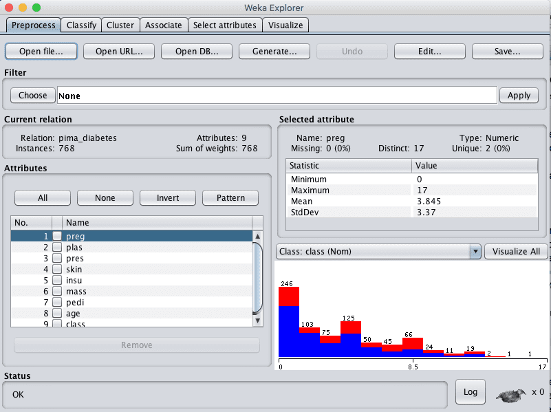
The dataset is now loaded into Weka.

Weka Load Pima Indians Onset of Diabetes Dataset

2. Analyze the Dataset

It is important to review your data before you start modeling.

Reviewing the distribution of each attribute and the interactions between attributes may shed light on specific data transforms and specific modeling techniques that we could use.

Summary Statistics

Review the details about the dataset in the “Current relation” pane. We can notice a few things:

• The dataset has the name pima_diabetes.
• There are 768 instances in the dataset. If we evaluate models using 10-fold cross validation then each fold will have about 76 instances, which is fine.
• There are 9 attributes, 8 input and one output attributes.

Click on each attribute in the “Attributes” pane and review the summary statistics in the “Selected attribute” pane.

We can notice a few facts about our data:

• The input attributes are all numerical and have differing scales. We may see some benefit from either normalizing or standardizing the data.
• There are no missing values marked.
• There are values for some attributes that do not seem sensible, specifically: plas, pres, skin, insu, and mass have values of 0. These are probably missing data that could be marked.
• The class attribute is nominal and has two output values meaning that this is a two-class or binary classification problem.
• The class attribute is unbalanced, 1 “positive” outcome to 1.8 “negative” outcomes, nearly double the number of negative cases. We may benefit from balancing the class values.

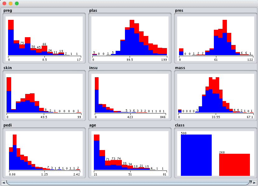
Attribute Distributions

Click the “Visualize All” button and lets review the graphical distribution of each attribute.

Weka Pima Indians Univariate Attribute Distributions

We can notice a few things about the shape of the data:

• Some attributes have a Gaussian-like distribution such as plas, pres, skin and mass, suggesting methods that make this assumption could achieve good results, like Logistic Regression and Naive Bayes.
• We see a lot of overlap between the classes across the attribute values. The classes do not seem easily separable.
• We can clearly see the class imbalance graphically depicted.

Attribute Interactions

Click the “Visualize” tab and lets review some interactions between the attributes.

1. Increase the window size so all plots are visible.
2. Increase the “PointSize” to 3 to make the dots easier to see.
3. Click the “Update” button to apply the changes.

Weka Pima Indians Scatter Plot Matrix

Looking across the graphs for the input variables, we can generally see poor separation between the classes on the scatter plots. This dataset will not be a walk in the park.

It suggests that we could benefit from some good data transforms and creating multiple views of the dataset. It also suggests we may get benefits from using ensemble methods.

3. Prepare Views of the Dataset

We noted in the previous section that this may be a difficult problem and that we may benefit from multiple views of the data.

In this section we will create varied views of the data, so that when we evaluate algorithms in the next section we can get an idea of the views that are generally better at exposing the structure of the classification problem to the models.

We are going to create 3 additional views of the data, so that in addition to the raw data we will have 4 different copies of the dataset in total. We will create each view of the dataset from the original and save it to a new file for later use in our experiments.

Normalized View

The first view we will create is of all the input attributes normalized to the range 0 to 1. This may benefit multiple algorithms that can be influenced by the scale of the attributes, like regression and instance based methods.

1. In the explorer with the data/diabetes.arff file loaded.
2. Click the “Choose” button in the “Filter” pane and choose the “unsupervised.attribute.Normalize” filter.
3. Click the “Apply” button to apply the filter.
4. Click each attribute in the “Attributes” pane and review the min and max values in the “Selected attribute” pane to confirm they are 0 and 1.
5. Click the “Save…” button, navigate to a suitable directory and type in a suitable name for this transformed dataset, such as “diabetes-normalize.arff”.
6. Close the Explorer interface to avoid contaminating the other views we want to create.

Weka Normalize Pima Indian Dataset

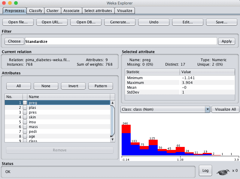
Standardized View

We noted in the previous section that some of the attribute have a Gaussian-like distribution. We can rescale the data and take this distribution into account by using a standardizing filter.

This will create a copy of the dataset where each attribute has a mean value of 0 and a standard deviation (mean variance) of 1. This may benefit algorithms in the next section that assume a Gaussian distribution in the input attributes, like Logistic Regression and Naive Bayes.

1. Open the Weka Explorer.
2. Load the Pima Indians onset of diabetes dataset.
3. Click the “Choose” button in the “Filter” pane and choose the “unsupervised.attribute.Standardize” filter.
4. Click the “Apply” button to apply the filter.
5. Click each attribute in the “Attributes” pane and review the mean and standard deviation values in the “Selected attribute” pane to confirm they are 0 and 1 respectively.
6. Click the “Save…” button, navigate to a suitable directory and type in a suitable name for this transformed dataset, such as “diabetes-standardize.arff“.
7. Close the Explorer interface.

Weka Standardize Pima Indians Dataset

Missing Data

In the previous section we suspected some of the attributes had bad or missing data marked with 0 values.

We can create a new copy of the dataset with the missing data marked and then imputed with an average value for each attribute. This may help methods that assume a smooth change in the attribute distributions, such as Logistic Regression and instance based methods.

First let’s mark the 0 values for some attributes as missing.

1. Open the Weka Explorer.
2. Load the Pima Indians onset of diabetes dataset.
3. Click the “Choose” button for the Filter and select the unsupervized.attribute.NumericalCleaner filter.
4. Click on the filter to configure it.
5. Set the attributeIndices to 2-6
6. Set minThreshold to 0.1E-8 (close to zero), which is the minimum value allowed for each attribute.
7. Set minDefault to NaN, which is unknown and will replace values below the threshold.
8. Click the “OK” button on the filter configuration.
9. Click the “Apply” button to apply the filter.
10. Click each attribute in the “Attributes” pane and review the number of missing values for each attribute. You should see some non-zero counts for attributes 2 to 6.

Weka Numeric Cleaner Data Filter For Pima Indians Dataset

Now, let’s impute the missing values as the mean.

1. Click the “Choose” button in the “Filter” pane and select unsupervised.attribute.ReplaceMissingValues filter.
2. Click the “Apply” button to apply the filter your dataset.
3. Click each attribute in the “Attributes” pane and review the number of missing values for each attribute. You should see all attributes should have no missing values and the distribution of attributes 2 to 6 should have changed slightly.
4. Click the “Save…” button, navigate to a suitable directory and type in a suitable name for this transformed dataset, such as “diabetes-missing.arff”.
5. Close the Weka Explorer.

Other views of the data you may want to consider investigating are subsets of features chosen by a feature selection method and a view where the class attribute is rebalanced.

4. Evaluate Algorithms

Let’s design an experiment to evaluate a suite of standard classification algorithms on the different views of the problem that we created.

1. Click the “Experimenter” button on the Weka GUI Chooser to launch the Weka Experiment Environment.

2. Click “New” to start a new experiment.

3. In the “Datasets” pane click “Add new…” and select the following 4 datasets:

• data/diabetes.arff (the raw dataset)
• diabetes-normalized.arff
• diabetes-standardized.arff
• diabetes-missing.arff

4. In the “Algorithms” pane click “Add new…” and add the following 8 multi-class classification algorithms:

• rules.ZeroR
• bayes.NaiveBayes
• functions.Logistic
• functions.SMO
• lazy.IBk
• rules.PART
• trees.REPTree
• trees.J48

5. Select IBK in the list of algorithms and click the “Edit selected…” button.

6. Change “KNN” from “1” to “3” and click the “OK” button to save the settings.

Weka Algorithm Comparison Experiment for Pima Indians Dataset

7. Click on “Run” to open the Run tab and click the “Start” button to run the experiment. The experiment should complete in just a few seconds.

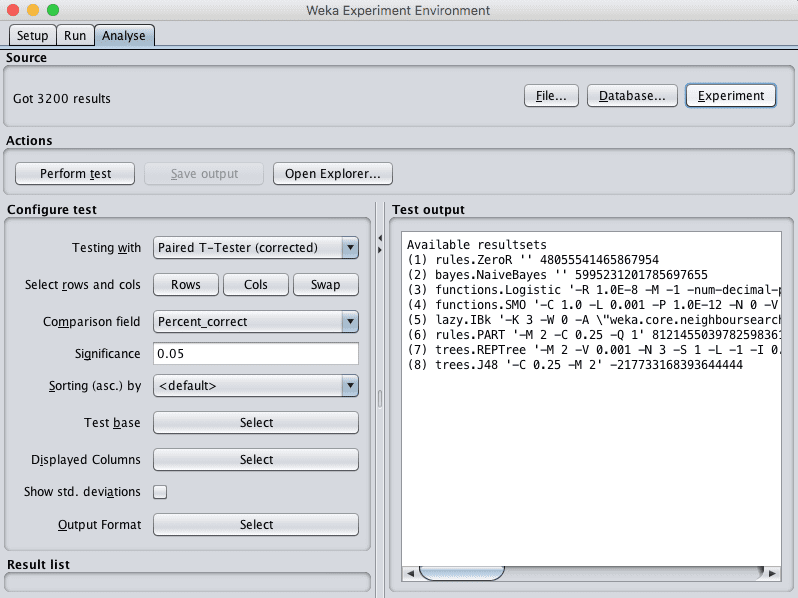
8. Click on the “Analyse” to open the Analyse tab. Click the “Experiment” button to load the results from the experiment.

Weka Load Algorithm Comparison Experiment Results for Pima Indians Dataset

9. Click the the “Perform test” button to perform a pairwise test-test comparing all of the results to the results for ZeroR.

We can see that all of the algorithms are skillful on all of the views of the dataset compared to ZeroR. We can also see that our baseline for skill is 65.11% accuracy.

Just looking at the raw classification accuracies, we can see that the view of the dataset with missing values imputed looks to have resulted in lower model accuracy in general. It also looks like there is little difference between the standardized and normalized results as compared to the raw results other than a few fractions of percent. It suggests we can probably stick with the raw dataset.

Finally, it looks like Logistic regression may have achieved higher accuracy results than the other algorithms, lets check if the difference is significant.

10. Click the “Select” button for “Test base” and choose “functions.Logistic”. Click the “Perform test” button to rerun the analysis.

It does look like the logistic regression results are better than some of the other results, such as IBk, PART, REPTree and ZeroR, but not statistically significantly different from NaiveBayes, SMO or J48.

11. Check “Show std. deviations” to show standard deviations.

12. Click the “Select” button for “Displayed Columns” and choose “functions.Logistic”, click “Select” to accept the selection. This will only show results for the logistic regression algorithm.

13. Click “Perform test” to rerun the analysis.

We now have a final result we can use to describe our model.

We can see that the estimated accuracy of the model on unseen data is 77.47% with a standard deviation of 4.39%.

14. Close the Weka Experiment Environment.

5. Finalize Model and Present Results

We can create a final version of our model trained on all of the training data and save it to file.

1. Open the Weka Explorer and load the data/diabetes.arff dataset.
2. Click on the Classify.
3. Select the functions.Logistic algorithm.
4. Change the “Test options” from “Cross Validation” to “Use training set”.
5. Click the “Start” button to create the final model.
6. Right click on the result item in the “Result list” and select “Save model”. Select a suitable location and type in a suitable name, such as “diabetes-logistic” for your model.

This model can then be loaded at a later time and used to make predictions on new data.

We can use the mean and standard deviation of the model accuracy collected in the last section to help quantify the expected variability in the estimated accuracy of the model on unseen data.

We can generally expect that the performance of the model on unseen data will be 77.47% plus or minus (2 * 4.39)% or 8.78%. We can restate this as between 68.96% and 86.25% accurate.

What is surprising about this final statement of model accuracy is that at the lower end, the model is only a shade better than the ZeroR model that achieved an accuracy if 65.11% by predicting a negative outcome for all predictions.

Summary

In this post you completed a binary classification machine learning project end-to-end using the Weka machine learning workbench.

Specifically, you learned:

• How to analyze your dataset and suggest at specific data transform and modeling techniques that may be useful.
• How to design and save multiple views of your data and spot check multiple algorithms on these views.
• How to finalize the model for making predictions on new data and presenting the estimated accuracy of the model on unseen data.

Do you have any questions about running a machine learning project in Weka or about this post? Ask your questions in the comments and I will do my best to answer them.

Discover Machine Learning Without The Code!

Develop Your Own Models in Minutes

...with just a few a few clicks

Discover how in my new Ebook:
Machine Learning Mastery With Weka

Covers self-study tutorials and end-to-end projects like:
Loading data, visualization, build models, tuning, and much more...

Finally Bring The Machine Learning To Your Own Projects

Skip the Academics. Just Results.

See What's Inside