
Autoregression is a time series model that uses observations from previous time steps as input to a regression equation to predict the value at the next time step.
It is a very simple idea that can result in accurate forecasts on a range of time series problems.
In this tutorial, you will discover how to implement an autoregressive model for time series forecasting with Python.
After completing this tutorial, you will know:
- How to explore your time series data for autocorrelation.
- How to develop an autocorrelation model and use it to make predictions.
- How to use a developed autocorrelation model to make rolling predictions.
Kick-start your project with my new book Time Series Forecasting With Python, including step-by-step tutorials and the Python source code files for all examples.
Let’s get started.
- Updated May/2017: Fixed small typo in autoregression equation.
- Updated Apr/2019: Updated the link to dataset.
- Updated Aug/2019: Updated data loading to use new API.
- Updated Sep/2019: Updated examples to use latest plotting API.
- Updated Apr/2020: Changed AR to AutoReg due to API change.

Autoregression Models for Time Series Forecasting With Python
Photo by Umberto Salvagnin, some rights reserved.
Autoregression
A regression model, such as linear regression, models an output value based on a linear combination of input values.
For example:
|
1 |
yhat = b0 + b1*X1 |
Where yhat is the prediction, b0 and b1 are coefficients found by optimizing the model on training data, and X is an input value.
This technique can be used on time series where input variables are taken as observations at previous time steps, called lag variables.
For example, we can predict the value for the next time step (t+1) given the observations at the last two time steps (t-1 and t-2). As a regression model, this would look as follows:
|
1 |
X(t+1) = b0 + b1*X(t-1) + b2*X(t-2) |
Because the regression model uses data from the same input variable at previous time steps, it is referred to as an autoregression (regression of self).
Stop learning Time Series Forecasting the slow way!
Take my free 7-day email course and discover how to get started (with sample code).
Click to sign-up and also get a free PDF Ebook version of the course.
Autocorrelation
An autoregression model makes an assumption that the observations at previous time steps are useful to predict the value at the next time step.
This relationship between variables is called correlation.
If both variables change in the same direction (e.g. go up together or down together), this is called a positive correlation. If the variables move in opposite directions as values change (e.g. one goes up and one goes down), then this is called negative correlation.
We can use statistical measures to calculate the correlation between the output variable and values at previous time steps at various different lags. The stronger the correlation between the output variable and a specific lagged variable, the more weight that autoregression model can put on that variable when modeling.
Again, because the correlation is calculated between the variable and itself at previous time steps, it is called an autocorrelation. It is also called serial correlation because of the sequenced structure of time series data.
The correlation statistics can also help to choose which lag variables will be useful in a model and which will not.
Interestingly, if all lag variables show low or no correlation with the output variable, then it suggests that the time series problem may not be predictable. This can be very useful when getting started on a new dataset.
In this tutorial, we will investigate the autocorrelation of a univariate time series then develop an autoregression model and use it to make predictions.
Before we do that, let’s first review the Minimum Daily Temperatures data that will be used in the examples.
Minimum Daily Temperatures Dataset
This dataset describes the minimum daily temperatures over 10 years (1981-1990) in the city Melbourne, Australia.
The units are in degrees Celsius and there are 3,650 observations. The source of the data is credited as the Australian Bureau of Meteorology.
Download the dataset into your current working directory with the filename “daily-min-temperatures.csv“.
The code below will load the dataset as a Pandas Series.
|
1 2 3 4 5 6 |
from pandas import read_csv from matplotlib import pyplot series = read_csv('daily-min-temperatures.csv', header=0, index_col=0) print(series.head()) series.plot() pyplot.show() |
Running the example prints the first 5 rows from the loaded dataset.
|
1 2 3 4 5 6 7 |
Date 1981-01-01 20.7 1981-01-02 17.9 1981-01-03 18.8 1981-01-04 14.6 1981-01-05 15.8 Name: Temp, dtype: float64 |
A line plot of the dataset is then created.
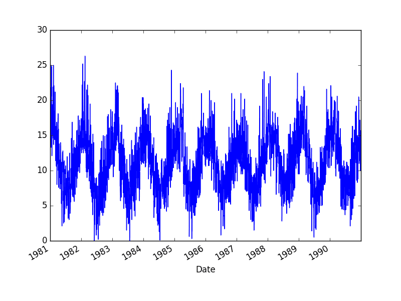
Minimum Daily Temperature Dataset Plot
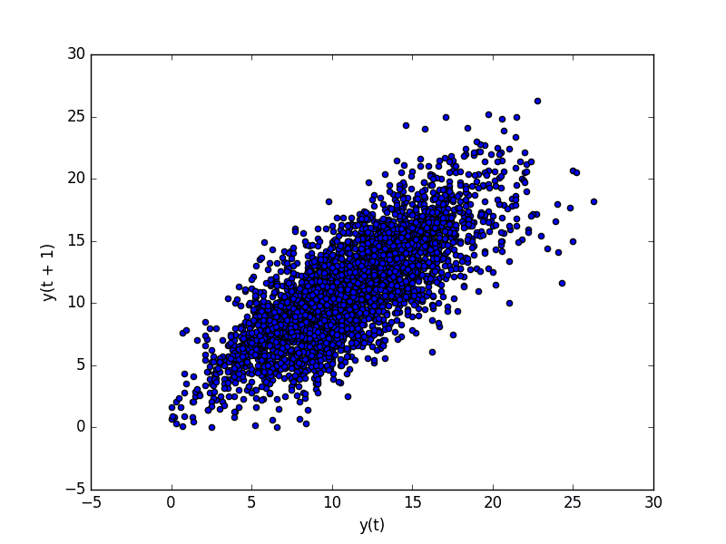
Quick Check for Autocorrelation
There is a quick, visual check that we can do to see if there is an autocorrelation in our time series dataset.
We can plot the observation at the previous time step (t-1) with the observation at the next time step (t+1) as a scatter plot.
This could be done manually by first creating a lag version of the time series dataset and using a built-in scatter plot function in the Pandas library.
But there is an easier way.
Pandas provides a built-in plot to do exactly this, called the lag_plot() function.
Below is an example of creating a lag plot of the Minimum Daily Temperatures dataset.
|
1 2 3 4 5 6 |
from pandas import read_csv from matplotlib import pyplot from pandas.plotting import lag_plot series = read_csv('daily-min-temperatures.csv', header=0, index_col=0) lag_plot(series) pyplot.show() |
Running the example plots the temperature data (t) on the x-axis against the temperature on the previous day (t-1) on the y-axis.
Minimum Daily Temperature Dataset Lag Plot
We can see a large ball of observations along a diagonal line of the plot. It clearly shows a relationship or some correlation.
This process could be repeated for any other lagged observation, such as if we wanted to review the relationship with the last 7 days or with the same day last month or last year.
Another quick check that we can do is to directly calculate the correlation between the observation and the lag variable.
We can use a statistical test like the Pearson correlation coefficient. This produces a number to summarize how correlated two variables are between -1 (negatively correlated) and +1 (positively correlated) with small values close to zero indicating low correlation and high values above 0.5 or below -0.5 showing high correlation.
Correlation can be calculated easily using the corr() function on the DataFrame of the lagged dataset.
The example below creates a lagged version of the Minimum Daily Temperatures dataset and calculates a correlation matrix of each column with other columns, including itself.
|
1 2 3 4 5 6 7 8 9 10 |
from pandas import read_csv from pandas import DataFrame from pandas import concat from matplotlib import pyplot series = read_csv('daily-min-temperatures.csv', header=0, index_col=0) values = DataFrame(series.values) dataframe = concat([values.shift(1), values], axis=1) dataframe.columns = ['t-1', 't+1'] result = dataframe.corr() print(result) |
This is a good confirmation for the plot above.
It shows a strong positive correlation (0.77) between the observation and the lag=1 value.
|
1 2 3 |
t-1 t+1 t-1 1.00000 0.77487 t+1 0.77487 1.00000 |
This is good for one-off checks, but tedious if we want to check a large number of lag variables in our time series.
Next, we will look at a scaled-up version of this approach.
Autocorrelation Plots
We can plot the correlation coefficient for each lag variable.
This can very quickly give an idea of which lag variables may be good candidates for use in a predictive model and how the relationship between the observation and its historic values changes over time.
We could manually calculate the correlation values for each lag variable and plot the result. Thankfully, Pandas provides a built-in plot called the autocorrelation_plot() function.
The plot provides the lag number along the x-axis and the correlation coefficient value between -1 and 1 on the y-axis. The plot also includes solid and dashed lines that indicate the 95% and 99% confidence interval for the correlation values. Correlation values above these lines are more significant than those below the line, providing a threshold or cutoff for selecting more relevant lag values.
|
1 2 3 4 5 6 |
from pandas import read_csv from matplotlib import pyplot from pandas.plotting import autocorrelation_plot series = read_csv('daily-min-temperatures.csv', header=0, index_col=0) autocorrelation_plot(series) pyplot.show() |
Running the example shows the swing in positive and negative correlation as the temperature values change across summer and winter seasons each previous year.
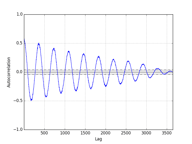
Pandas Autocorrelation Plot
The statsmodels library also provides a version of the plot in the plot_acf() function as a line plot.
|
1 2 3 4 5 6 |
from pandas import read_csv from matplotlib import pyplot from statsmodels.graphics.tsaplots import plot_acf series = read_csv('daily-min-temperatures.csv', header=0, index_col=0) plot_acf(series, lags=31) pyplot.show() |
In this example, we limit the lag variables evaluated to 31 for readability.
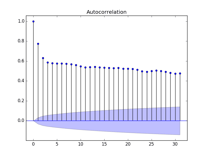
Statsmodels Autocorrelation Plot
Now that we know how to review the autocorrelation in our time series, let’s look at modeling it with an autoregression.
Before we do that, let’s establish a baseline performance.
Persistence Model
Let’s say that we want to develop a model to predict the last 7 days of minimum temperatures in the dataset given all prior observations.
The simplest model that we could use to make predictions would be to persist the last observation. We can call this a persistence model and it provides a baseline of performance for the problem that we can use for comparison with an autoregression model.
We can develop a test harness for the problem by splitting the observations into training and test sets, with only the last 7 observations in the dataset assigned to the test set as “unseen” data that we wish to predict.
The predictions are made using a walk-forward validation model so that we can persist the most recent observations for the next day. This means that we are not making a 7-day forecast, but 7 1-day forecasts.
|
1 2 3 4 5 6 7 8 9 10 11 12 13 14 15 16 17 18 19 20 21 22 23 24 25 26 27 28 29 30 31 |
from pandas import read_csv from pandas import DataFrame from pandas import concat from matplotlib import pyplot from sklearn.metrics import mean_squared_error series = read_csv('daily-min-temperatures.csv', header=0, index_col=0) # create lagged dataset values = DataFrame(series.values) dataframe = concat([values.shift(1), values], axis=1) dataframe.columns = ['t-1', 't+1'] # split into train and test sets X = dataframe.values train, test = X[1:len(X)-7], X[len(X)-7:] train_X, train_y = train[:,0], train[:,1] test_X, test_y = test[:,0], test[:,1] # persistence model def model_persistence(x): return x # walk-forward validation predictions = list() for x in test_X: yhat = model_persistence(x) predictions.append(yhat) test_score = mean_squared_error(test_y, predictions) print('Test MSE: %.3f' % test_score) # plot predictions vs expected pyplot.plot(test_y) pyplot.plot(predictions, color='red') pyplot.show() |
Running the example prints the mean squared error (MSE).
The value provides a baseline performance for the problem.
|
1 |
Test MSE: 3.423 |
The expected values for the next 7 days are plotted (blue) compared to the predictions from the model (red).
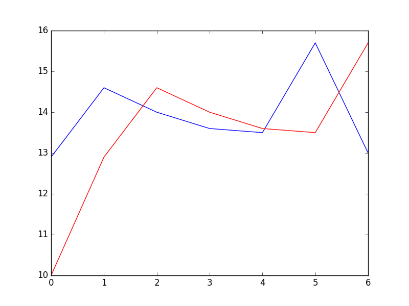
Predictions From Persistence Model
Autoregression Model
An autoregression model is a linear regression model that uses lagged variables as input variables.
We could calculate the linear regression model manually using the LinearRegession class in scikit-learn and manually specify the lag input variables to use.
Alternately, the statsmodels library provides an autoregression model where you must specify an appropriate lag value and trains a linear regression model. It is provided in the AutoReg class.
We can use this model by first creating the model AutoReg() and then calling fit() to train it on our dataset. This returns an AutoRegResults object.
Once fit, we can use the model to make a prediction by calling the predict() function for a number of observations in the future. This creates 1 7-day forecast, which is different from the persistence example above.
The complete example is listed below.
|
1 2 3 4 5 6 7 8 9 10 11 12 13 14 15 16 17 18 19 20 21 22 23 24 25 |
# create and evaluate a static autoregressive model from pandas import read_csv from matplotlib import pyplot from statsmodels.tsa.ar_model import AutoReg from sklearn.metrics import mean_squared_error from math import sqrt # load dataset series = read_csv('daily-min-temperatures.csv', header=0, index_col=0, parse_dates=True, squeeze=True) # split dataset X = series.values train, test = X[1:len(X)-7], X[len(X)-7:] # train autoregression model = AutoReg(train, lags=29) model_fit = model.fit() print('Coefficients: %s' % model_fit.params) # make predictions predictions = model_fit.predict(start=len(train), end=len(train)+len(test)-1, dynamic=False) for i in range(len(predictions)): print('predicted=%f, expected=%f' % (predictions[i], test[i])) rmse = sqrt(mean_squared_error(test, predictions)) print('Test RMSE: %.3f' % rmse) # plot results pyplot.plot(test) pyplot.plot(predictions, color='red') pyplot.show() |
Running the example the list of coefficients in the trained linear regression model.
The 7 day forecast is then printed and the mean squared error of the forecast is summarized.
|
1 2 3 4 5 6 7 8 9 10 11 12 13 14 15 16 |
Coefficients: [ 5.57543506e-01 5.88595221e-01 -9.08257090e-02 4.82615092e-02 4.00650265e-02 3.93020055e-02 2.59463738e-02 4.46675960e-02 1.27681498e-02 3.74362239e-02 -8.11700276e-04 4.79081949e-03 1.84731397e-02 2.68908418e-02 5.75906178e-04 2.48096415e-02 7.40316579e-03 9.91622149e-03 3.41599123e-02 -9.11961877e-03 2.42127561e-02 1.87870751e-02 1.21841870e-02 -1.85534575e-02 -1.77162867e-03 1.67319894e-02 1.97615668e-02 9.83245087e-03 6.22710723e-03 -1.37732255e-03] predicted=11.871275, expected=12.900000 predicted=13.053794, expected=14.600000 predicted=13.532591, expected=14.000000 predicted=13.243126, expected=13.600000 predicted=13.091438, expected=13.500000 predicted=13.146989, expected=15.700000 predicted=13.176153, expected=13.000000 Test RMSE: 1.225 |
A plot of the expected (blue) vs the predicted values (red) is made.
The forecast does look pretty good (about 1 degree Celsius out each day), with big deviation on day 5.
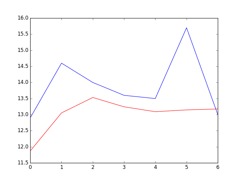
Predictions From Fixed AR Model
The statsmodels API does not make it easy to update the model as new observations become available.
One way would be to re-train the AutoReg model each day as new observations become available, and that may be a valid approach, if not computationally expensive.
An alternative would be to use the learned coefficients and manually make predictions. This requires that the history of 29 prior observations be kept and that the coefficients be retrieved from the model and used in the regression equation to come up with new forecasts.
The coefficients are provided in an array with the intercept term followed by the coefficients for each lag variable starting at t-1 to t-n. We simply need to use them in the right order on the history of observations, as follows:
|
1 |
yhat = b0 + b1*X1 + b2*X2 ... bn*Xn |
Below is the complete example.
|
1 2 3 4 5 6 7 8 9 10 11 12 13 14 15 16 17 18 19 20 21 22 23 24 25 26 27 28 29 30 31 32 33 34 35 36 |
# create and evaluate an updated autoregressive model from pandas import read_csv from matplotlib import pyplot from statsmodels.tsa.ar_model import AutoReg from sklearn.metrics import mean_squared_error from math import sqrt # load dataset series = read_csv('daily-min-temperatures.csv', header=0, index_col=0, parse_dates=True, squeeze=True) # split dataset X = series.values train, test = X[1:len(X)-7], X[len(X)-7:] # train autoregression window = 29 model = AutoReg(train, lags=29) model_fit = model.fit() coef = model_fit.params # walk forward over time steps in test history = train[len(train)-window:] history = [history[i] for i in range(len(history))] predictions = list() for t in range(len(test)): length = len(history) lag = [history[i] for i in range(length-window,length)] yhat = coef[0] for d in range(window): yhat += coef[d+1] * lag[window-d-1] obs = test[t] predictions.append(yhat) history.append(obs) print('predicted=%f, expected=%f' % (yhat, obs)) rmse = sqrt(mean_squared_error(test, predictions)) print('Test RMSE: %.3f' % rmse) # plot pyplot.plot(test) pyplot.plot(predictions, color='red') pyplot.show() |
Again, running the example prints the forecast and the mean squared error.
|
1 2 3 4 5 6 7 8 |
predicted=11.871275, expected=12.900000 predicted=13.659297, expected=14.600000 predicted=14.349246, expected=14.000000 predicted=13.427454, expected=13.600000 predicted=13.374877, expected=13.500000 predicted=13.479991, expected=15.700000 predicted=14.765146, expected=13.000000 Test RMSE: 1.204 |
We can see a small improvement in the forecast when comparing the error scores.
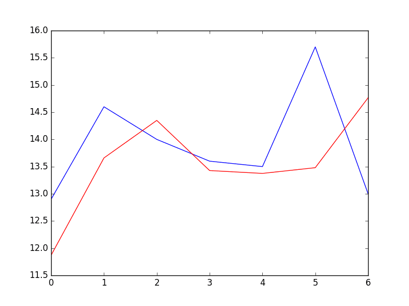
Predictions From Rolling AR Model
Further Reading
This section provides some resources if you are looking to dig deeper into autocorrelation and autoregression.
- Autocorrelation on Wikipedia
- Autoregressive model on Wikipedia
- Chapter 7 – Regression-Based Models: Autocorrelation and External Information, Practical Time Series Forecasting with R: A Hands-On Guide.
- Section 4.5 – Autoregressive Models, Introductory Time Series with R.
Summary
In this tutorial, you discovered how to make autoregression forecasts for time series data using Python.
Specifically, you learned:
- About autocorrelation and autoregression and how they can be used to better understand time series data.
- How to explore the autocorrelation in a time series using plots and statistical tests.
- How to train an autoregression model in Python and use it to make short-term and rolling forecasts.
Do you have any questions about autoregression, or about this tutorial?
Ask your questions in the comments below and I will do my best to answer.
Want to Develop Time Series Forecasts with Python?

Develop Your Own Forecasts in Minutes
...with just a few lines of python codeDiscover how in my new Ebook:
Introduction to Time Series Forecasting With Python
It covers self-study tutorials and end-to-end projects on topics like: Loading data, visualization, modeling, algorithm tuning, and much more...
Finally Bring Time Series Forecasting to
Your Own Projects
Skip the Academics. Just Results.


Thank you Jason for the awesome article
In case anyone hits the same problem I had –
I downloaded the data from the link above as a csv file.
It was failing to be imported due to three rows in the temperature column containing ‘?’.
Once these were removed the data imported ok.
Thanks for the heads up Gary.
hi man , what do you think the best model that can deal with hour
There are no best algorithms. I recommend testing a suite of methods in order to discover what works best for your specific dataset.
Hey Jason, thanks for the article. How would you go about forecasting from the end of the file when expected value is not known?
Hi Tim, you can use mode.predict() as in the example and specify the index of the time step to be predicted.
Hey Jason, I am not clear with the use of model.predict(). If you could help me on this in predicting the values for the next 10 days if the model has learned the values till today.
Sure, see this post:
https://machinelearningmastery.com/make-sample-forecasts-arima-python/
Hi Jason,
Thanks for all of your wonderful blogs. They are really helping a lot. One question regarding this post is that I believe that AR modeling also presume that time series is stationary as the observations should be i.i.d. .Does that AR function from statsmodels library checks for stationary and use the de-trended de-seasonalized time series by itself if required? Also, if we use sckit learn library for AR model as you described do we need to check for and make adjustments by ourselfs for this?
Hi Farrukh, great question.
The AR in statsmodels does assume that the data is stationary.
If your data is not stationary, you must make it stationary (e.g. differencing and other transforms).
Thanks for the answer. Though we did not conduct proper test here for trend/seasonal stationarity check in the example above but from figure apparently it seems like that there is a seasonal effect. So in that case whether applying AR model is good to go?
Great question Farrukh.
AR is designed to be used on stationary data, meaning data with no seasonal or trend information.
Or to be specific, is it OK to apply AR model direct here on the given data without checking the seasonality and removing it if present which is showing some signs in first graph apparently?
Hi. I am working on something similar and i have the same question? in the above AR model, the normal non transformed time series has been used and it has not been made stationary? is that correct and applicable?
It is a good idea to make the series stationary before using an AR model.
Dear Dr Jason,
I had a go at the ‘persistence model’ section.
The dataset I used was the sp500.csv dataset.
From your code
As soon as I try to compute the “test_score”, I get the following error,
Any idea,
Anthony of Sydney NSW
It looks like you need to convert your data to floating point values.
E.g. in numpy this might be:
Dear Dr Jason,
Fixed the problem. You cannot assume that all *.csv numbers are floats or ints. For some reason, the numbers seem to be enclosed in quotes. Note that the data is is for the sp500.csv not the above exercise.
Note the numbers in the output are enclosed in quotes:
It works now,
Regards
Anthony from Sydney
Glad to hear you fixed it Anthony.
Dear Dr Jason,
The problem has been fixed. The values in the array were strings, so I had to convert them to strings.
So I converted the strings in each array to float.
Hope that helps others trying to convert values to appropriate data types in order to do numerical calculations.
Anthony from Sydney NSW
how can I show my prediction as date, instead of log, for example I have data set incident number for each week, I want to predict the following week
week1 669
week2 443
week3 555
so on april week 1 I want to show time series the prediction of week1 week2 of April
Sorry, I’m not sure I understand. Perhaps you can give a fuller example of inputs and outputs?
Thanks for this wonderful tutorial. I discovered your articles on facebook last year. Since then I have been following all your tutorials and I must confess that, though I started learning about machine learning in less than a year, my knowledge base has tremendously increased as a result of this free services you have been posting for all to see on the website.
Thanks once more for this generosity Dr Jason.
My question is that, I have carefully followed all your procedures in this article on my data set that was recorded every 10mins for 2 months. Please I would like to know which time lag is appropriate for forecasting to see the next 7 days value or more or less.
My time series is a stationary one according to the test statistics and histogram I have applied on it. but I still don’t know if a reasonable conclusion can be reached with a data set that was recorded for 2 months every 10mins daily.
Well done on your progress!
This post gives you some ideas on how to select suitable q and p values (lag vars):
https://machinelearningmastery.com/gentle-introduction-autocorrelation-partial-autocorrelation/
I hope that helps as a start.
Dr Jason,
Thank you so much for this post. I have finally learned how to go from theory to practice.
I’m so glad to hear that Soy, thanks!
Dr Jason, How do i predict the low and high confidence interval of prediction of an AR model?
This post will help:
https://machinelearningmastery.com/time-series-forecast-uncertainty-using-confidence-intervals-python/
Thanks for the reply. It was a very good post. But, it was for ARIMA model. I am having some problem with the ARIMA model I cannot use it. Is there such a confidence interval forecasting for AR model?
Yes, I believe the same approach applies. Use the forecast() function.
ValueError: On entry to DLASCL parameter number 4 had an illegal value
I ma found above error when i use
model = AR(train) ## no error
model_fit = model.fit() ## show above error
Thanks for the great write-up Jason. One question though , I am interested in doing an autoregression on my timeseries data every nth days. For example. Picking the first 20 days and predicting the value of the 20th day. Then picking the next 20 days (shift 1 over) and predict the value of the 21st day and so forth until the end of my dataset. How can this be achieved in code? Thanks.
Consider using a variation of walk forward validation:
https://machinelearningmastery.com/backtest-machine-learning-models-time-series-forecasting/
Hi Jason,
Thanks for your article. I have few doubts.
1) We do analysis on the autocorrelation plots and auto-correlation function only after making the time series stationary right?
2) For the time series above, the correlation value is maximum for lag=1. So is it like the value at t-1 is given more weight while doing Autoregression?
3) When the AR model says, for lag-29 model the MSE is minimum. Does it mean the regression model constructed with values from t to t-29 gave minimum MSE?
Please clarify.
Thank you
1. Ideally, yes, analysis after the data is stationary.
2. Yes.
3. Yes.
Thanks.
You’re welcome.
Hey Jason. Thanks for the awesome tutorial.
in this line…
print(‘Lag: %s’ % model_fit.k_ar)
print(‘Coefficients: %s’ % model_fit.params)
What is the “layman” explanation of what lag and coeffcients are?
Is it that “lag” is what the AR model determined that the significance ends (i.e. after this number, the autocorrelation isn’t “strong enough) and that the coeff. are the p-value of null hypotehsis on “intensity” of the autocorrelation?
Lag observations are observations at prior time steps.
Lag coefficients are the weightings on those lag observations.
Thank you Jason. That answer has still gotten me more confused. 🙂
The section where you manually calculate the predictions.. you’re specifying history.append(obs). So does this mean that the test data up to t0 is required to predict t1?
In another words, this model can only predict 1 time period away ?
If I am wrong, how do I tweak the code to predict up to n periods away?
i think i answered my own after reading this… https://machinelearningmastery.com/multi-step-time-series-forecasting/
Example you gave with statsmodels.tsa.ar_model.AR is for single step prediction, am I correct?
Correct, but the forecast() function for ARIMA (and maybe AR) can make a multi-step forecast. It might just not be very good.
Dear Jason
Thanks for this wonderful guideline. I have a problem with my dataset and I am digging in time series modeling.
I try to model a physical model such that
y(t+1) = y(t) + f(a(t), b(t), c(t)) with AR models.
Actually problem is predict metal temperature using basic heat transfer where y means metal Temperature and f is a function of some sensors data like coolant mass flow rate, coolant temperaute, gas flowrate and gas temperatue.
Which model do you advise to use?
Sounds like a great problem. I would recommend testing a suite of different methods to see what works best for your specific data, given your specific modeling requirements.
I recommend this process generally:
https://machinelearningmastery.com/start-here/#process
Hi Jason…
I read your few articles and found very helpful. I am very new to machine learning and would like to ask the meaning of these prediction points such as predicted=14.349246 so what is the meaning of this value does it mean???
how does it help to understanding the prediction?
please post about cross regression also if you have posted any.
Sorry, I don’t follow. Perhaps you can rephrase your question?
Thanks for the wonderful article.
I have a question: How can we make a prediction based on multiple columns by AR?
For an example, there are columns of
Date, Pricing, ABC, PQR
ABC, PQR contribute in predicting prices. So I want to predict pricing based on these columns as well.
Thank you
It may be possible, but I do not have a worked example, sorry.
How could you make this a Deep Autoregressive Network with Keras?
A deep MLP will do the trick!
Thank you for the amazing tutorial
I have a question though. According to Pandas’ Autocorrelation plot, the maximum correlation is gained when lag=1. But the AR model selects lag=29 to build the autoregression.
I checked this code on my dataset, and the autoregression with lag=1 performed much better on test case that lag=14 chosen by AR model. Can you explain this? I thought that autocorrelation checks for linear relationship, thus, the autoregression which maps a linear function to the data should naturally perform best on the lag variable giving the maximum Pearson correlation.
Perhaps the method was confused by noise in the data or small sample size?
What if time is also included along with the date?
1981-01-01,20.7 is like 1981-01-01 03:00:00,20.7
Sure.
Hi great tutorial. Just wanted to ask how would I change the order or lag in the code? Also if you had any tutorials for understanding how to use the statsmodels library.
My book is the best source of material on the topic:
https://machinelearningmastery.com/introduction-to-time-series-forecasting-with-python/
You can either difference your code directly or use the d parameter in the ARIMA model to control the differencing order. I have tutorials on both, perhaps start here:
https://machinelearningmastery.com/start-here/#timeseries
Thanks a lot! I ran into a problem while developing the AR model when some of the dates were dropped. I had to mention the frequency parameter even though I was already supplying the date-times
Interesting. Did it fix your issues?
Hi Jason,
Excellent article! Any chance of a blog post on how to do vector autoregression with big data? Sometimes an LSTM is overkill, and even a vanilla RNN can be overkill, so something with just plain old autoregression would be great.
The VAR package in Python does this, but it runs into memory issues very quickly with large, sparse datasets.
If you know of any other tools for vector autoregression, any insight you have would be appreciated!
Thanks for the suggestion Carolyn.
Dear Jason,
Thank you so much for your wonderful article. I have a doubt regarding Data driven forecasting. I need to forecast appliance energy which depends upon 26 variables.I have data of appliance energy along with 26 variables of 3 months. With the help of 26 variables How can I forecast appliance energy for future?
Good question.
You can transform the data into a supervised learning problem and try a suite of machine learning algorithms:
https://machinelearningmastery.com/convert-time-series-supervised-learning-problem-python/
I hope to provide more information on this topic in the future.
Hey Jason!
Thank you for the article. I have a doubt regarding this. How can I make predictions for future dates, that are not present in the dataset?
Call model.predict() and specify the dates or index.
This tutorial will show you how:
https://machinelearningmastery.com/make-sample-forecasts-arima-python/
can you please provide me a detaile example over VAR model?
I hope to cover the method in the future, thanks for the suggestion.
from pandas import Series
from matplotlib import pyplot
series = Series.from_csv(‘G:\Study_Material\daily-minimum-temperatures.csv’)
print(series.head())
series.plot()
pyplot.show()
ha an error as : Empty ‘DataFrame’: no numeric data to plot
how to resolve it sir?
Perhaps double check you have loaded the data correctly?
Its a wonderful post that I came across and thanks a lot putting up great content with great examples. I am new to machine learning and I have a question regarding the use of ARIMA for sparse timeseries. I have events that can recur every day, week, once a few weeks, or monthly. Typical example of this could be business meetings. Different meetings could happen at different frequencies. Is it appropriate to use ARIMA for predicting the underlying pattern. My real world problem involves predicting the size of virtual meetings based on their past history. Lets assume a service like hangout. I am trying to see if ARIMA would be an appropriate algorithm for predicting resource requirement for a virtual meeting based on its history. I tried ARIMA based on this tutorial but the results weren’t convincing. I wasn’t sure if its appropriate to model this problem as a time series problem and is ARIMA a good choice for such problems.
Perhaps try it as a starting point.
I’m trying to work out o AR model to forecast a series using a lag of 192.
The series has a datapoint every 15 min but the you receive the data, the day after it was measured.
So you have to forecast the next day (D+1) with data of the previous day (D-1) hence a lag of 192 in datapoints that are 15 min apart.
Is there a way to contrain the AR() function to all datapoints before t-192 ?
Perhaps fit a regularized linear regression model directly on your chosen lags?
Thanks for your reply!
Were can I find some more information about a regularized lineair regression model ?
Any good book on machine learning, for example:
https://amzn.to/2KSoQ0a
Thanks a lot for this lovely article
Thanks, I’m happy it helped.
Hi Dr. Brownlee,
Fantastic article — I’m following along step by step and it’s helping.
at the step:
model.fit()
I get this error:
TypeError: Cannot find a common data type.
Where could this come from?
That is odd. Are you using the code and data from the tutorial?
Did you replace the “?” chars in the data file?
Shouldn’t your first equation be:
X(t) = b0 + b1*X(t-1) + b2*X(t-2)
Instead of:
X(t+1) = b0 + b1*X(t-1) + b2*X(t-2)
Then where is “t”?
I have the same question as Phil, and I’m not sure what you mean by the answer. When you wrote: “we can predict the value for the next time step (t+1) given the observations at the last two time steps (t-1 and t-2)”, the last two time steps for (t+1) are t, t-1 not t-1 and t-2.
Why did you jump over t?
also, in the following sentence you said it the right way:
“We can plot the observation at the previous time step (t-1) with the observation at the next time step (t+1) as a scatter plot.”
So you are talking of current time (t) vs previous step (t-1) vs next step (t+1).
That’s why I don’t think the formula should be as Phil mentioned.
Yes, thanks.
Hi Jason. Great job with your blog and this article!
I was wondering if you could help me with the following question: in your example, you choose 7 points as your test set and the AR model has a lower MSE for these points than the persistence model. However, if I make the test set larger, say a couple hundred points, and make AR predictions, I get a higher MSE with the AR model. I know a couple hundred points means like a year of data points and the AR model could be updated in between to obtain better results, but I was just wondering what is your view on this matter. Does it mean that the AR model is not suitable for predictions too far in the future?
Also, if I use the AR model for predicting about 180 points, AR’s MSE value rises quite significantly, to roughly 9. Interestingly, if the test set is enlarged even more to about 350 points, MSE value falls to about 7. Persistence model’s MSE has lower variability. What does this changing MSE say about the data and applying AR to it?
The further you predict into the future, the worse the performance.
Hello Dr. Jason Brownlee,
Thanks a lot for your excellent article.
I have a question related to predicted results.
Why the predicted solution at i-th point is very close the expected solution at (i-1)-th point ?
In all most your article, I have seen this.
I don’t understand why? Can you help me answer this question, please?
Thank you so much Dr Jason Brownlee.
Best,
Dieu Do
This is a common question that I answer here:
https://machinelearningmastery.com/faq/single-faq/why-is-my-forecasted-time-series-right-behind-the-actual-time-series
Hi Jason, thanks for your sharing.
I am trying to use AR model to predict a complex-valued time series. I used a series as below and replace the tempreature data in your example code:
series = Series([1, 1+1j, 2, 3, 4, 5, 8, 1+2j, 3, 5])
However, it reports an error message like this:
/anaconda/lib/python3.6/site-packages/statsmodels/tsa/tsatools.py in lagmat(x, maxlag, trim, original, use_pandas)
377 dropidx = nvar
378 if maxlag >= nobs:
–> 379 raise ValueError(“maxlag should be < nobs")
380 lm = np.zeros((nobs + maxlag, nvar * (maxlag + 1)))
381 for k in range(0, int(maxlag + 1)):
ValueError: maxlag should be < nobs
Please shed a light on how to correct it.
Thanks.
The error suggests you may need to change the configuration of the model to suite your data.
Hello,
In the section “Quick Check for Autocorrelation”, you shifted the data by one position back and you named the columns ‘t-1’ and ‘t+1’. In the article ‘https://machinelearningmastery.com/convert-time-series-supervised-learning-problem-python/’ in the section ‘Pandas shift() Function’ you have the code line: ‘df[‘t-1’] = df[‘t’].shift(1)’ that is shifted by one means 1 time difference(t-1, t). Can you explain which one is correct? What point have I missed?
Thanks
Really it should be ‘t’ and ‘t-1.
Hi Dr. Brownlee,
I have used your tutorial to make some predictions on a dataset which records every minute the number of used parking spaces for 2017. For the Persistence model I get a test MSE score of 12.7 and for the Autoregression model a test MSE score of 74. Could you tell me if it is good or bad? In the meantime, could you give me more details on how the MSE results work on your code does it run on the entire dataset?
Regards.
Good or bad is only knowable in comparison to the persistence model.
You can answer this question yourself.
74 > 12 == bad.
Hi Dr. Brownlee,
Is there any references and example code of NARX (Non-Linear AutoRegressive with eXogenous inputs) ? I apologize if this is out of topic probably you have experience about this
regards,
I’m not sure, sorry.
When we say that a given model makes use of lag value of 3, which one of the followings is the given model equation:
X(t) = b0 + b1*X(t-1) + b2*X(t-2)+ b3*X(t-3)
X(t) = b0 + b3*X(t-3)
I assume it’s the first one, but I’m not sure.
It will be a linear function of three prior time steps to the step being predictions.
The specifics of the linear function will vary across algorithms.
Hi Jason,
How can I change the order for the AR model using this code.
E.g. AR(1), AR(2) etc?
Create the AR model and provide an integer for the order.
I don’t really understand what you mean?
I’d just like to know how to do it based on the example you gave. Wouldn’t it just be a single line where I add the extra parameter as ‘order number’?
model = AR(train, order = 1)
would it be like that, based on the code above
Yes, use maxlag on the fit() function or use an ARIMA without d or q elements.
I see, yes, you set the “maxlag” argument on the call to fit(). More here:
http://www.statsmodels.org/devel/generated/statsmodels.tsa.ar_model.AR.fit.html#statsmodels.tsa.ar_model.AR.fit
Alternately, you can use an ARIMA and set the order as (n, 0, 0).
Could you please explain why it’s not “cheating”, so to speak, to append the observation at a time step to the history list. Isn’t this equivalent to feeding the model part of the data it is trying to predict? Is this possible in real life situations where we may not know the actual value of the thing we are trying to predict? I am referring to line 26 in the code which generates the “Predictions From Rolling AR Model.” I will appreciate it you could enlighten me about this please. Thank you.
No.
It is called walk-forward validation and under this model we are assuming that the true observation becomes available after the prediction was made, and in turn can be used by the model.
If this assumption does not hold for your data, you can design a walk forward validation strategy that captures the assumptions for your specific forecast problem.
More on walk forward validation here:
https://machinelearningmastery.com/backtest-machine-learning-models-time-series-forecasting/
Thank you. That helped resolve my uncertainty.
Hi,
model.predict(start , end) always gives me the same value and I end up getting a straight line prediction. So I used the history method shown above and kept adding yhat to test for the number of out of sample predictions I wanted (code below). Is it correct?
for t in range(len(test)+number_of_values_to_predict):
length = len(history)
lag = [history[i] for i in range(length-window,length)]
yhat = coef[0]
for d in range(window):
yhat += coef[d+1] * lag[window-d-1]
obs = test[t]
predictions.append(yhat)
history.append(obs)
test = np.append(test,yhat)
I’m not really sure what you’re trying to achieve?
I am trying to achieve out of sample forecasting like forecasting the value for the next 7 days. Using predict() gives me the same predicted value and gives me a straight line prediction. Hence I tried to use the code above. Do you think it is correct to do that?
Perhaps try a different model or use different data?
Hey Jason,
You are only providing an autoregression model in a case that you only have one label or one input which is previous records of the same output. What if for example we are concerned about the prediction of energy consumption of a house and we have different input labels like inddor temp, outdoor temp and taking into considertion the home architecture and previous records.
How can we develop such a model?
do you have an example for that?
Thank you
Good question, I refer to this as a multivariate time series problem, and you can find examples here:
https://machinelearningmastery.com/start-here/#deep_learning_time_series
Hey Jason, I’m following your tutorial using my own dataset. But I have some questions about the results. (1)what does the Lag , that is the value of model_fit.k_ar, mean for your dataset?(2)what is the meaning of the period of Figure “Pandas Autocorrelation Plot” ? Could you take a moment to tell me something about them? Thank you very much.
Lag is a prior observation, perhaps this will help:
https://machinelearningmastery.com/time-series-forecasting-supervised-learning/
More about autocorrelation here:
https://machinelearningmastery.com/gentle-introduction-autocorrelation-partial-autocorrelation/
Could you please explain the relation between the Lag(model_fit.k_ar) and the period of dataset?
How so?
or how can I get the period of the time series dataset except Fast Fourier Transform?
I see, you could review a plot of the series.
You could use domain knowledge.
You could use a grid search on a simple polynomial function.
Hi
Thanks for this useful article. Where can I get the data file “daily-minimum-temperatures.csv”? I can’t reach the target site when I click on “Learn more about the dataset here”.
Thanks
You can download it directly from here:
https://raw.githubusercontent.com/jbrownlee/Datasets/master/daily-min-temperatures.csv
got it, thanks for your hlep
Hi Jason,
Quick question here. Why do we start the train dataset at 1 and not 0?
In your code we have: train, test = X[1:len(X)-7], X[len(X)-7:]
But having this instead: train, test = X[:len(X)-7], X[len(X)-7:] would allow the model to train on 1 more value (starting at index 0 instead of starting at index 1).
Thanks. Not sure what I was thinking there…
Hi Jason,
what order is the AR model in the code?
Or in what way is the order defined?
Order is the number of lag observations considered by the model.
You can grid search different values or use an ACF/PACF plot to choose the value.
Hi Jason,
I am new to python, is it the update issue of pandas?
I cannot run the code for “Quick Check for Autocorrelation :”
unless adding the below 2 line of code
Data[‘Date’] = pd.to_datetime(Data[‘Date’])
series=pd.Series(Data[‘Temp’])
lag_plot(series)
pyplot.show()
thank you
Sorry to hear that, what problem were you having exactly?
I have some suggestions here that might help:
https://machinelearningmastery.com/faq/single-faq/why-does-the-code-in-the-tutorial-not-work-for-me
Hi Jason,
Thank you for the tutorial, very helpful. I have a question though
How is your last example (rolling forecast) different to what statsmodels.tsa.ar_model.AR.predict() would do when dynamic=False?
The way I understand it, it would do what you did in your last example, but you are getting different results, so not sure what I am missing.
From statsmodels website:
“The dynamic keyword affects in-sample prediction. If dynamic is False, then the in-sample lagged values are used for prediction. If dynamic is True, then in-sample forecasts are used in place of lagged dependent variables. The first forecasted value is start.”
Thanks.
I believe dynamic only effects “in sample” data, e.g. data within the scope of the training data.
Hi Jason,
Thank you for the tutorial, very helpful. I have a question though
You wrote that “the statsmodels library provides an autoregression model that automatically selects an appropriate lag value using statistical tests and trains a linear regression model.”
Is it using any model selection criteria like AIC, BIC to select the appropriate lag value or is it approximating all the models and picking the one with the least MSE?
fit([maxlag, method, ic, trend, …])
Could you please explain what all inputs we’re giving in this in your example. What is the maxlag, method and ic when we do model.fit( )?
maxlag is the maximum input lag to consider when fitting the model.
The other parameters are described here:
http://www.statsmodels.org/stable/generated/statsmodels.tsa.ar_model.AR.fit.html#statsmodels.tsa.ar_model.AR.fit
Thanks, I’m glad it helped.
Good question, you can see more about how it works here:
http://www.statsmodels.org/stable/generated/statsmodels.tsa.ar_model.AR.fit.html#statsmodels.tsa.ar_model.AR.fit
Hey Jason,
Do you know what the methods are for validating AR model?
Specific tests that could be done to show the model developed in valid
Yes, walk-forward validation:
https://machinelearningmastery.com/backtest-machine-learning-models-time-series-forecasting/
Hi Jason,
Thank you for the tutorial, very helpful. I have a question that your ACF lag is big in this case and so as I. How can we decide to choose the ARIMA parameters if the lag of ACF or PACF is very big ? In my case , my ACF decay towards to zero at lag 1000, and PACF at lag 30.
Great question, I give some general advice for choosing ARIMA parameters from ACF/PACF plots here:
https://machinelearningmastery.com/gentle-introduction-autocorrelation-partial-autocorrelation/
Thank you for the article.
Isn’t partial autocorrelation (PACF) plot supposed to be used to determine the statistically significant lag cofficients for an AR model. Isn’t ACF used for the Moving average part, not the AR part of an ARMA model? I was confused by the choice of using the ACF plot for the AR part of the model
See this tutorial:
https://machinelearningmastery.com/gentle-introduction-autocorrelation-partial-autocorrelation/
Hi Jason. Very nice and clear explanation.
Thanks!
Hi Jason, I was wondering if this technique of lag variables could be used for other features. So it seems like above you are predicting weather so you are using lag variables of weather data. What if we wanted to use lag variables of another variable such as total sunlight per day. Even though this is a different variable can you use the say technique in terms of lagging data to predict weather?
Yes, it can be useful for any time series data.
Hi Jason
I am trying to do a dynamic forecast using OLS. The model has an AR(1) variable and n exdog variables.
I use a for loop to run the regression many times for different combinations of the exdog variables and store the results. I split into test/train sets and run a prediction on the test set and store the MAE and RMSE.
The problem I have is the out of sample test is using the actual lagged AR(1) variable rather than dynamically generating it. I want to use the realized values of the exdog variables but the dynamically estimated AR(1) variable.
Do you have any thoughts on the best way of doing this please? I have looked at SARIMAX as an alternative but wanted to use OLS ideally.
Also which of your books would you recommend for statsmodels/OLS/time series forecasting?
Do you also have anything on monte carlo in python?
Cheers
Mark
I don’t follow the specific problem you’re having sorry. “generated” do you mean predicted as in a recursive model?
I cover the basics of time series forecasting with ARIMA in this book (no exog or sarima though):
https://machinelearningmastery.com/introduction-to-time-series-forecasting-with-python/
Not much on MC in python:
https://machinelearningmastery.com/monte-carlo-sampling-for-probability/
And:
https://machinelearningmastery.com/markov-chain-monte-carlo-for-probability/
Thanks of the links Jason.
I mean the standard way OLS works with statsmodels.predict() is to do a fixed forecast using the actual lagged dependent variables in the test data if there is a AR term in the equation. For a true out of sample forecast, for a given assumed exog data set or scenario, I want the forecast to be dynamic with regard to the AR term in the equation. Otherwise it looks better at out of sample forecasting than it really is.
I don’t follow, sorry. Perhaps you can rephrase your question/issue?
Hi Mark amazing tutorial many thanks,
When using plot_acf(series, lags=30), I don’t see why the autocorrelation plot appears 2 times.
Is there a bug?
Thank you in advance for your reply.
Mark?
Sorry to hear that you’re having trouble, perhaps this will help:
https://machinelearningmastery.com/faq/single-faq/why-does-the-code-in-the-tutorial-not-work-for-me
Hi Jason :), who said Mark :P,
Thanks a lot, solved 🙂
You did in your comment:
“Hi Mark amazing tutorial many thanks,”
Happy to hear you solved your problem.
Hi,
Can we fit Support vector regression instead of linear regression ?
If possible , then what is the procedure and how we can get the residuals from SVR-AR(1) model ?
Looking forward to hearing from you soon.
Best,
Arabzai
Yes, use this to prepare your data:
https://machinelearningmastery.com/convert-time-series-supervised-learning-problem-python/
Hi, do you know what statistical method statsmodels.tsa.ar_model.AR( ) uses under the hood to determine the optimal order for the AR? (Can’t seem to find anything on the documentation.)
If not, are there any models you recommend me reading up on? I appreciate that you can observe an ACF and qualitatively decide a rough number.
The AR model does not optimize the order, you must specify the order when calling the fit() function.
You can use a grid search to tune the model on your data, here is an example:
https://machinelearningmastery.com/grid-search-arima-hyperparameters-with-python/
If the AR model doesn’t optimise the order, then where does model.fit.k_ar come from?
In the tutorial:
model = AR(train)
model_fit = model.fit( )
print(“Lag: %s” % model_fit.k_ar)
>>> Lag: 29
Where does the lag of 29 come from?
looks like it tests different lag values using a configured criterion, learn more here:
https://www.statsmodels.org/stable/generated/statsmodels.tsa.ar_model.AR.fit.html#statsmodels.tsa.ar_model.AR.fit
Thank you so much Jason, you saved my day
You’re welcome!
Hello,
I am trying to follow the precedure, but I am having problems with statsmodels. All my dependencies are upto date, but I cannot import statsmodels, raising the error:
ImportError: cannot import name ‘assert_equal’ from ‘statsmodels.compat.pandas’
Do you know what am I supposed to do?
Thanks
Perhaps confirm that pandas and statsmodels are up to date again?
My versions are:
I wanted to ask is AR(lags=10) model is equal to an ARMA(10,0)
Yes, I would expect so.
hi how can i know numbre off the correct lag?
If you’re unsure test a suite of values and use a number of lag obs that results in a model with the best performance.
Hi, Would you recommend using “statsmodels.tsa.ar_model.ar_select_order” to select best lag periods as “statsmodels.tsa.ar_model.AR” is now depreciated?
I’m not familiar with statsmodels.tsa.ar_model.ar_select_order
AutoReg is an appropriate replacement:
https://www.statsmodels.org/stable/generated/statsmodels.tsa.ar_model.AutoReg.html
Nice example. This one helped me to start my VAR model project. Here, I’m using multivariate time series and statsmodel’s VAR model. As you mentioned the API won’t update the coefficients for new observations. Since it’s a multivariate time series, what can I do get the prediction for a long time (say 6 months)?
I believe you can call forecast() and predict as long as you like.
Then re-fit the model as you get new data.
In most practical cases, we have some “regressable” variables in addition to the time series.
Variables that are not uniformly periodic (seasonal) and generally in our control. eg. In a retail store sales forecasting application, “gift promotion scheme on (Y/N)” or “scheme discount percentage offered (% or $)” may be significantly affecting the output variable, sales. Just running a timeseries model will ignore the effects of the schemes. How are these situations to be handled?
They can be included as exogenous variables to a linear model.
When I run
from pandas import read_csv
from matplotlib import pyplot
from statsmodels.tsa.ar_model import AutoReg
from sklearn.metrics import mean_squared_error
from math import sqrt
# load dataset
series = read_csv(‘daily-minimum-temperatures.csv’, header=0, index_col=0, parse_dates=True, squeeze=True)
# split dataset
X = series.values
train, test = X[1:len(X)-7], X[len(X)-7:]
# train autoregression
model = AutoReg(train, lags=29)
I get the following error
—————————————————————————
TypeError Traceback (most recent call last)
in
11 train, test = X[1:len(X)-7], X[len(X)-7:]
12 # train autoregression
—> 13 model = AutoReg(train, lags=29)
14 model_fit = model.fit()
15 print(‘Coefficients: %s’ % model_fit.params)
~/anaconda3/lib/python3.7/site-packages/statsmodels/tsa/ar_model.py in __init__(self, endog, lags, trend, seasonal, exog, hold_back, period, missing)
163 hold_back=None, period=None, missing=’none’):
164 super(AutoReg, self).__init__(endog, exog, None, None,
–> 165 missing=missing)
166 self._trend = string_like(trend, ‘trend’,
167 options=(‘n’, ‘c’, ‘t’, ‘ct’))
~/anaconda3/lib/python3.7/site-packages/statsmodels/tsa/base/tsa_model.py in __init__(self, endog, exog, dates, freq, missing, **kwargs)
44 def __init__(self, endog, exog=None, dates=None, freq=None,
45 missing=’none’, **kwargs):
—> 46 super(TimeSeriesModel, self).__init__(endog, exog, missing=missing,
47 **kwargs)
48
TypeError: super(type, obj): obj must be an instance or subtype of type
Sorry to hear that.
This may help:
https://machinelearningmastery.com/faq/single-faq/why-does-the-code-in-the-tutorial-not-work-for-me
Hi Jason, thanks for the article.
I have a question, in the istruction AutoReg(train, lags=29) the lags parameter is equal to 29 because in the ACF graph we notice that there is a strong correlation up to 29 time?
Wouldn’t it be better to consider the PACF graph?
Thank you for your answer.
Correct.
See this on ACF/PACF plots:
https://machinelearningmastery.com/gentle-introduction-autocorrelation-partial-autocorrelation/
Hi,
Nice explanation but I want to clarify that the time lags t-1 refers to one lag of time and the current time you are referring to is t+1. Then why don’t you take it as t and t+1 or t-1 and t.
I know this is a very basic question but Appreciate your answer on it.
It is a good idea, I should do that.
Hi Jason,
Thanks for very nice article. I am trying to perform the following , could you please suggest/guide me.
My original data is like below
Month Price
2011-01-01 1405.07
2011-02-01 408.58
2011-03-01 277.75
2011-04-01 294.81
2011-05-01 511.77
2011-06-01 515.90
I have to predict the price (by regression) considering lag of 5, with the rebuilt the data set as below I need to predict the value for 5th element (X)
Dataset = [1405,408,277,294,X]
[408,277,294,511,X]
[277,294,511,515,X]
How I can achieve the same?
Thanks in advance
-Girish
Perhaps get started with time series forecasting generally here:
https://machinelearningmastery.com/start-here/#timeseries
hi,
I want a code for EEG signal prediction with autoregressive model , so what should be the changes in this temperature prediction .I am doing in jupyter notebook with MNE and Pandas.
Please help me.
Perhaps try developing an ARIMA or SARIMA model for your dataset and compare the results to other methods.
This might be a good place to start:
https://machinelearningmastery.com/start-here/#timeseries
Sir it’s my project. I want code for EAR model to do my project. So I was searching for AR model related to EEG and to modify AR to EAR but I am not getting code related to EEG .can u help me.
Sorry, I cannot write code for you.
Perhaps you can adapt an example on the blog for your specific dataset.
sir,
I tried with EEG dataset with your autoregressive code and the output is fully different from expected and predicted values . Any solution?
Perhaps try some data preparation?
Perhaps try an alternate configuration?
Perhaps try an alternate model?
Hello Jason,
Do you know how to modify the model set up so that we can put constraints on the coefficient matrix A? For example, in VAR(1), Yt = (A1) (Yt-1) + E, A1= [a11, a12; a21, a22], how to impose a21 = 0 since I already know one granger cause the other, but not the other way around before running the model? I also want granger causality test to reflect that too. Do you know the solution?
Thanks
Not off hand, sorry. It may require custom code.
Thanks so much for the useful primer! I found lines 18-30 of the final code chunk a bit more verbose than necessary, in part because history ends up being an array of 1-length arrays rather than a flat array.
I rewrote that chunk as follows to get the same output:
history = train[len(train)-window:].flatten()

predictions = list()

for (t, obs) in enumerate(test.flatten()):

hist_len = len(history)

lag = np.concatenate(([1.0], np.flip(history[hist_len-window:])))

prediction = np.dot(coef, lag)

predictions.append(prediction)

history = np.append(history, obs)

print('predicted=%f, expected=%f' % (prediction, obs))
You’re welcome.
Thanks for sharing!
Hi Jason,
Can we have scenario generations with this method? I mean several stochastic scenarios.
Thanks
Yes, there are many examples on the blog, you can use the search box.
Thank you for this. Really good explanation of the AR model given that the article is 4yrs old. I do have a question tho, I have beed using the ARIMA function on statsmodel, the lags and order the same? Meaning you are using the autocorrelations of the past 29 time series to predict the next value? So this comes out as an AR(29) model?
If you’re referring to one of the example there, you’re correct.
Thank you for this great tutorial.
Please either correct the filename in the code pieces to read the CSV file
series = read_csv(‘daily-minimum-temperatures.csv’, header=0, index_col=0)
or rename the CSV file itself (currently: daily-min-temperatures.csv) to make filenames consistent and therefore avoiding Python error to not find the file.
Took me a little bit of time to realize why Python couldn’t find the file after downloading and putting in the working directory.
Thanks.
Good catch. Thanks!
Hi,
I would like to get the weights of this model. But model.weights is not working with this specific model. Could you tell a way to obtain the weights of this model.
There are not weights in the model but there are coefficients. See the line: “print(‘Coefficients: %s’ % model_fit.params)”
Hey! First of all Thank you for your articles and guides you really helped me a lot.
My question is, we constructed a model here and our forecast looks really good. But can you explain how that walk forward method works. I will write what I understand so please tell me if I’m right.
We fit our model and get coefficients first. And we have a set of train data with the size of window and it is at the end of train data which is called history. After that we started a loop for test set size and inside that loop, we get lag set and it is history set at first then we manually predict I don’t get why didn’t we just use forecast() function but anyway we did that and we original value of predicted value to train set and continue so we keep predicting with only last 29 data and didn’t change our model. I hope that’s how it works.
What I don’t get is what’s the point of that? We don’t change our model we don’t fit again what’s the point? We keep using same coefficients. That just shows how well our model is trained and it only predicts 1 value everytime. Why don’t we just go and predict upcoming 7 data instead doing this?
Hi Enes…Please see the following regarding your questions around walk forward validation:
https://machinelearningmastery.com/backtest-machine-learning-models-time-series-forecasting/
Hi just leaving my thanks for the article. Best wishes.
Pablo
Great feedback Pablo!
One question.
In the persistence model, why do you define the function model_persistence(x)? When it does nothing but return the same value? You can plot test_X and test_y and it would be the same graph? Is it for notation/explanation only?
Hi Pablo…You are correct. It serves just as an illustration.
Hello Jason, Many thanks again for the wonderful guideline. In the alternative where learned coefficients are used to manually make predictions. How can the code be modified to test out of sample ?
Hi Jason,
Thank you for the article.
Snippet from your code:
model = AutoReg(train, lags=29)
model_fit = model.fit()
How did you determine lags = 29?
Is any way to let Statsmodels determine the best no for lags?
You might add model_fit.aic to evaluate the model.
Hi Sophia…You may want to investigate hyperparameter optimization techniques.
https://machinelearningmastery.com/combined-algorithm-selection-and-hyperparameter-optimization/
HI JASON
I have six variables to predict water consumption.
ID,MONTHLY CONSUMPTION,YEAR,CUSTOMER TYPE, POPULATION.
My question is how i write the independent and dependent variables using regression model?
Hi James,
Thanks a lot, it was pretty helpfull.
So, if i understood correctly, what you call “rolling AR Model” is only rolling for the the validation on the test set, but your training set is only one, right?
What do you think about fitting in a rolling-training-window? Do you have some code examples for that?
Thanks again!
Hi Isadora…You are very welcome! Your understanding of “rolling AR Model” is correct!
The following resource provides many code samples that will add clarity:
https://machinelearningmastery.com/introduction-to-time-series-forecasting-with-python/
Hi there,
Is there a way to get the standard errors for the static and dynamic AR forecasts? Like in R the predict function for AR models has a ‘prediction’ element and a ‘standard error’ element so that you can plot the confidence intervals along with the prediction.
This has been super helpful so far, thank you.
Hi Izzy…Some ideas in the following resource may be of interest to you:
https://www.geeksforgeeks.org/how-to-plot-a-confidence-interval-in-python/
Hi Jason,
How did you come up with the lag=29?
Hi Amir…The following resource provides another example of how “lags” may be chosen:
https://towardsdatascience.com/how-to-use-an-autoregressive-ar-model-for-time-series-analysis-bb12b7831024
Jason this is all very helpful! I was curious why using the learned coefficents for prediction would provide results (as defined by a RMSE of 1.204) slightly closer than the initial AutoRegression predictions (RMSE 1.225). Is that a normal expected behavior when running this type of analysis?
Hi Jeremy…Thank you for your feedback! Variations are expected as such models are stocastic.
https://machinelearningmastery.com/stochastic-optimization-for-machine-learning/
Hi Jason, thank you so much for your helpful courses. Implementing AutoReg model, I receive different estimation values for same input data. Do you know its reason? Thank you so much.
Hi Reza…this resource may add clarity:
https://machinelearningmastery.com/stochastic-in-machine-learning/
Hi Jason, thank you so much for the link. According to wiki, there are two general ways to estimate the parameters of AR model as 1) Yule–Walker equations and 2) MLE. I am familiar with the MLE method in which the parameters are estimated based on input data (stochastic). I mean, there is no random number generation within the parameters’ estimation (randomness) which you clearly explained them in the link provided. According to the MLE method, I expect that if I enter same data into AR model (train data, test data, and the order of AR), then I will get same estimation values. I am running the AR with same data more than one times, and obtain different estimation values. I am not sure if the estimation process uses the randomness (generate random number from normal distribution for example). Sorry for long writing.
Sorry again, in the MLE method, we are estimating the AR parameters based on given probability distribution and observed data. I did not set any statistical distribution as input. The observed data (train data, test data, and order of AR) is same in second time, but I get different results.
Thanks for the tutorial. However, i wish to know how predicted (yhat) values are realized manually using the expression. yhat = b0 + b1*X1 + b2*X2 … bn*Xn
Hi Walter…To retrieve the regression coefficients from an autoregressive (AR) model in a statistical software or programming environment, you can use built-in functions and methods provided by the library you are using. Here’s a step-by-step guide on how to do this in Python using the
statsmodelslibrary, which is a popular choice for statistical modeling and econometrics:### Using Python and
statsmodels1. **Install and Import Necessary Libraries**
First, make sure you have the necessary libraries installed (
numpy,pandas,matplotlib, andstatsmodels). You can install these usingpipif they’re not already installed:bash
pip install numpy pandas matplotlib statsmodels
Then, import these libraries in your Python script or notebook:
python

import numpy as np

import pandas as pd

import matplotlib.pyplot as plt

from statsmodels.tsa.ar_model import AutoReg
2. **Prepare Your Time Series Data**
You’ll need a time series dataset. Here, I’ll create a simple simulated time series data for demonstration purposes:
python

# Generate some time series data (e.g., random walk)

np.random.seed(0)

data = pd.Series(50 + np.random.normal(0, 1, 100).cumsum())
3. **Fit an Autoregressive Model**
Choose the appropriate number of lags based on domain knowledge, or use statistical methods such as ACF/PACF plots to determine it. For this example, I’ll assume we choose one lag:
python

# Fit an AR model

model = AutoReg(data, lags=1)

fitted_model = model.fit()
4. **Retrieve and Display the Coefficients**
The fitted model object contains the estimated coefficients, which include the intercept (if any) and the lag coefficients:
python

# Display the regression coefficients

print("Coefficients of the model:")

print(fitted_model.params)
This will print the coefficients, including the constant term (intercept) and the coefficients for each lag used in the model.
5. **Using the Coefficients for Further Analysis**
These coefficients can be used to understand the impact of past values on the current value in the series, or for making forecasts. Here’s how you might use these coefficients for prediction:
python# Make predictions
predictions = fitted_model.predict(start=len(data), end=len(data) + 5, dynamic=False)
# Plot the original data and the forecasts
plt.figure(figsize=(10, 5))
plt.plot(data, label='Original Data')
plt.plot(np.arange(len(data), len(data) + 6), predictions, label='Forecast', linestyle='--')
plt.legend()
plt.show()
### Additional Tips
– **Choosing the Number of Lags**: The choice of lags in an AR model is crucial. Too few lags might not capture the dynamics, while too many lags could lead to overfitting. Consider using statistical criteria like AIC or BIC for selection.
– **Checking Model Assumptions**: Always check for stationarity in your time series data before fitting an AR model. Non-stationary data can lead to spurious results.
By following these steps, you can effectively fit an AR model, retrieve its coefficients, and use them for forecasting or analysis. This methodology can be adapted to more complex models or different types of data as required.