An Introduction to Recurrent Neural Networks and the Math That Powers Them

When it comes to sequential or time series data, traditional feedforward networks cannot be used for learning and prediction. A mechanism is required to retain past or historical information to forecast future values. Recurrent neural networks, or RNNs for short, are a variant of the conventional feedforward artificial neural networks that can deal with sequential data and can be trained to hold knowledge about the past.

After completing this tutorial, you will know:

• Recurrent neural networks
• What is meant by unfolding an RNN
• How weights are updated in an RNN
• Various RNN architectures

Kick-start your project with my book Building Transformer Models with Attention. It provides self-study tutorials with working code to guide you into building a fully-working transformer model that can
translate sentences from one language to another...

Let’s get started.

An introduction to recurrent neural networks and the math that powers Them. Photo by Mehreen Saeed, some rights reserved.

Tutorial Overview

This tutorial is divided into two parts; they are:

1. The working of an RNN
   1. Unfolding in time
   2. Backpropagation through time algorithm
2. Different RNN architectures and variants

Prerequisites

This tutorial assumes that you are already familiar with artificial neural networks and the backpropagation algorithm. If not, you can go through this very nice tutorial, Calculus in Action: Neural Networks, by Stefania Cristina. The tutorial also explains how a gradient-based backpropagation algorithm is used to train a neural network.

What Is a Recurrent Neural Network

A recurrent neural network (RNN) is a special type of artificial neural network adapted to work for time series data or data that involves sequences. Ordinary feedforward neural networks are only meant for data points that are independent of each other. However, if we have data in a sequence such that one data point depends upon the previous data point, we need to modify the neural network to incorporate the dependencies between these data points. RNNs have the concept of “memory” that helps them store the states or information of previous inputs to generate the next output of the sequence.

Unfolding a Recurrent Neural Network

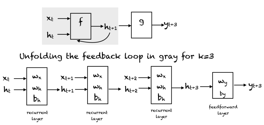
Recurrent neural network. Compressed representation (top), unfolded network (bottom).

A simple RNN has a feedback loop, as shown in the first diagram of the above figure. The feedback loop shown in the gray rectangle can be unrolled in three time steps to produce the second network of the above figure. Of course, you can vary the architecture so that the network unrolls $k$ time steps. In the figure, the following notation is used:

• $x_t \in R$ is the input at time step $t$. To keep things simple, we assume that $x_t$ is a scalar value with a single feature. You can extend this idea to a $d$-dimensional feature vector.
• $y_t \in R$ is the output of the network at time step $t$. We can produce multiple outputs in the network, but for this example, we assume that there is one output.
• $h_t \in R^m$ vector stores the values of the hidden units/states at time $t$. This is also called the current context. $m$ is the number of hidden units. $h_0$ vector is initialized to zero.
• $w_x \in R^{m}$ are weights associated with inputs in the recurrent layer
• $w_h \in R^{mxm}$ are weights associated with hidden units in the recurrent layer
• $w_y \in R^m$ are weights associated with hidden units to output units
• $b_h \in R^m$ is the bias associated with the recurrent layer
• $b_y \in R$ is the bias associated with the feedforward layer

At every time step, we can unfold the network for $k$ time steps to get the output at time step $k+1$. The unfolded network is very similar to the feedforward neural network. The rectangle in the unfolded network shows an operation taking place. So, for example, with an activation function f:

Hence, in the feedforward pass of an RNN, the network computes the values of the hidden units and the output after $k$ time steps. The weights associated with the network are shared temporally. Each recurrent layer has two sets of weights: one for the input and the second for the hidden unit. The last feedforward layer, which computes the final output for the kth time step, is just like an ordinary layer of a traditional feedforward network.

The Activation Function

We can use any activation function we like in the recurrent neural network. Common choices are:

• Sigmoid function: $\frac{1}{1+e^{-x}}$
• Tanh function: $\frac{e^{x}-e^{-x}}{e^{x}+e^{-x}}$
• Relu function: max$(0,x)$

Training a Recurrent Neural Network

The backpropagation algorithm of an artificial neural network is modified to include the unfolding in time to train the weights of the network. This algorithm is based on computing the gradient vector and is called backpropagation in time or BPTT algorithm for short. The pseudo-code for training is given below. The value of $k$ can be selected by the user for training. In the pseudo-code below, $p_t$ is the target value at time step t:

1. Repeat till the stopping criterion is met:
   1. Set all $h$ to zero.
   2. Repeat for t = 0 to n-k
      1. Forward propagate the network over the unfolded network for $k$ time steps to compute all $h$ and $y$
      2. Compute the error as: $e = y_{t+k}-p_{t+k}$
      3. Backpropagate the error across the unfolded network and update the weights

Types of RNNs

There are different types of recurrent neural networks with varying architectures. Some examples are:

One to One

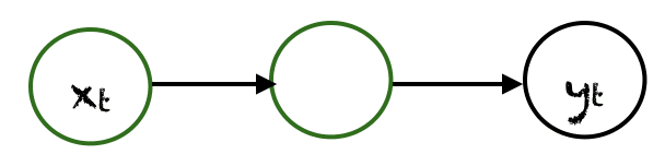
Here, there is a single $(x_t, y_t)$ pair. Traditional neural networks employ a one-to-one architecture.

One to Many

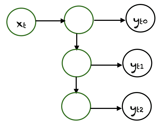
In one-to-many networks, a single input at $x_t$ can produce multiple outputs, e.g., $(y_{t0}, y_{t1}, y_{t2})$. Music generation is an example area where one-to-many networks are employed.

Many to One

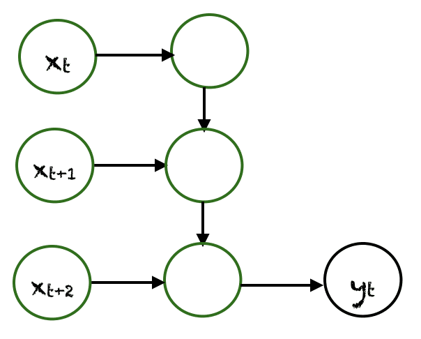
In this case, many inputs from different time steps produce a single output. For example, $(x_t, x_{t+1}, x_{t+2})$ can produce a single output $y_t$. Such networks are employed in sentiment analysis or emotion detection, where the class label depends upon a sequence of words.

Many to Many

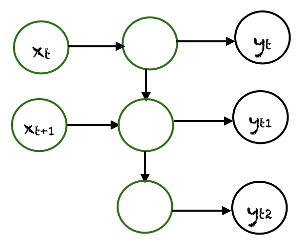
There are many possibilities for many-to-many. An example is shown above, where two inputs produce three outputs. Many-to-many networks are applied in machine translation, e.g., English to French or vice versa translation systems.

Advantages and Shortcomings of RNNs

RNNs have various advantages, such as:

• Ability to handle sequence data
• Ability to handle inputs of varying lengths
• Ability to store or “memorize” historical information

The disadvantages are:

• The computation can be very slow.
• The network does not take into account future inputs to make decisions.
• Vanishing gradient problem, where the gradients used to compute the weight update may get very close to zero, preventing the network from learning new weights. The deeper the network, the more pronounced this problem is.

Different RNN Architectures

There are different variations of RNNs that are being applied practically in machine learning problems:

Bidirectional Recurrent Neural Networks (BRNN)

In BRNN, inputs from future time steps are used to improve the accuracy of the network. It is like knowing the first and last words of a sentence to predict the middle words.

Gated Recurrent Units (GRU)

These networks are designed to handle the vanishing gradient problem. They have a reset and update gate. These gates determine which information is to be retained for future predictions.

Long Short Term Memory (LSTM)

LSTMs were also designed to address the vanishing gradient problem in RNNs. LSTMs use three gates called input, output, and forget gate. Similar to GRU, these gates determine which information to retain.

Further Reading

This section provides more resources on the topic if you are looking to go deeper.

Books

• Deep Learning Essentials by Wei Di, Anurag Bhardwaj, and Jianing Wei.
• Deep Learning by Ian Goodfellow, Joshua Bengio, and Aaron Courville.

Articles

• Wikipedia article on BPTT
• A Tour of Recurrent Neural Network Algorithms for Deep Learning
• A Gentle Introduction to Backpropagation Through Time

Summary

In this tutorial, you discovered recurrent neural networks and their various architectures.

Specifically, you learned:

• How a recurrent neural network handles sequential data
• Unfolding in time in a recurrent neural network
• What is backpropagation in time
• Advantages and disadvantages of RNNs
• Various architectures and variants of RNNs

Do you have any questions about RNNs discussed in this post? Ask your questions in the comments below, and I will do my best to answer.

Learn Transformers and Attention!

Teach your deep learning model to read a sentence

...using transformer models with attention

Discover how in my new Ebook:
Building Transformer Models with Attention

It provides self-study tutorials with working code to guide you into building a fully-working transformer models that can
translate sentences from one language to another...

Give magical power of understanding human language for
Your Projects

See What's Inside